The Definitive Guide to Real-Time PCR (RT-PCR): Principles, Quantification, and Clinical Diagnostics

1. Introduction: The Evolution of Molecular Amplification

The landscape of molecular biology was fundamentally altered by the development of the Polymerase Chain Reaction (PCR) by Kary Mullis in the mid-1980s. While Mullis’s original method allowed for the exponential amplification of nucleic acid sequences, it remained primarily an end-point, qualitative tool. The strategic shift toward Real-Time PCR (quantitative PCR or qPCR) was realized in 1992 by Higuchi et al., who introduced the continuous monitoring of the amplification process. This revolutionized quantitative nucleic acid analysis by shifting the diagnostic focus from the plateau phase to the exponential growth phase.

Real-Time PCR utilizes fluorescence to report the accumulation of DNA during the reaction’s active growth. By identifying the CT​ value (Cycle Threshold), laboratories can transition from binary “positive/negative” results to high-precision quantification. This capability is now a cornerstone of molecular diagnostics, enabling the detection of initial template amounts with a sensitivity often reaching a single molecule.

The core advantages of real-time molecular analysis include:

• Speed: Elimination of multi-day incubation periods, providing results within hours rather than weeks.

• Dynamic Range: Ability to quantify targets across a vast spectrum, typically exceeding five to six orders of magnitude.

• Accuracy and Reproducibility: High precision in determining the starting template quantity, minimizing the inter-assay variation common in end-point methods.

• Safety and Containment: Utilization of closed-tube systems to virtually eliminate the risk of post-PCR carry-over contamination.

Analytical Evolution: End-Point vs. Real-Time PCR

Category	End-Point PCR	Real-Time PCR (qPCR)
Product Monitoring	Analyzed only after the final cycle; limited by the plateau effect.	Monitored continuously (kinetics) during every cycle.
Quantification Ability	Qualitative/Semi-quantitative; most samples reach the same endpoint.	Highly accurate; enables absolute quantification of starting molecules.
Sensitivity	Limited by gel electrophoresis detection thresholds.	Exceptional; capable of detecting a single cell equivalent.

Anatomy of the Amplification Plot

The amplification plot visualizes the progression of the reaction where the X-axis denotes the Cycle Number and the Y-axis represents the Normalized Reporter Signal (ΔRn). In high-precision assays, Rn is a normalized value calculated as the ratio of the fluorescence emission intensity of the reporter dye (e.g., FAM) to the fluorescence of a passive reference dye, such as TAMRA. This normalization is critical to account for tube-to-tube variability and optical noise. The final value, ΔRn, is defined by the formula: ΔRn=(Rn+)−(Rn−), where Rn+ is the emission of the reporter at a given time and Rn− is the baseline emission measured prior to significant amplification.

A successful reaction follows three distinct phases:

1. Baseline/Background Phase: Typically occurring between cycles 1 and 15, the signal is “within the variability of the base-line data.” During these cycles, the nuclease activity has not yet cleaved enough probe to generate a signal that exceeds the background noise of the reagents.

2. Exponential (Log) Phase: This is the critical window for data collection. Here, the reaction is at peak efficiency, and the target sequence theoretically doubles with every cycle. Because reagents are not yet limiting, the time it takes to reach this phase is a direct reflection of the starting DNA concentration.

3. Plateau Phase: The signal eventually levels off as the reaction kinetics shift from exponential to linear growth and finally to a halt. This saturation is caused by the depletion of three critical components: primers, dNTPs, and reporter probes. Furthermore, the DNA polymerase itself may become limiting or lose activity, causing the reaction to “run out of steam.”

To compare these plots across different samples, we must establish a standardized “finish line” for the data.

The Three Pillars of Real-Time PCR Value are:

1. Contamination Control: The “closed-tube” system eliminates post-PCR handling, such as agarose gel electrophoresis or plate capture hybridization, virtually removing the risk of carry-over contamination.

2. Analytical Range: An unprecedented linear dynamic range (1,000,000-fold) enables the quantification of gene copy numbers from a single cell equivalent to millions of copies without re-dilution.

3. Efficiency: Compatibility with 96-well formats and automated sequence detectors like the ABI Prism 7700 maximizes throughput and reduces labor-intensive manual processing.

Real-time PCR remains the authoritative gold standard for quantitative nucleic acid analysis, providing the precision and reproducibility required for modern molecular diagnostics and clinical validation.

2. Theoretical Foundations: The RT-PCR Thermal Cycle and Components

Successful RT-PCR requires a meticulous orchestration of chemical components and thermal shifts. The physical process is defined by repetitive temperature cycles, but as a clinical director, one must look beyond the heat to the buffer chemistry.

The Essential Thermal Stages

• Denaturation (95°C): High temperature separates double-stranded DNA (dsDNA). Complete separation is vital; partially melted structures reanneal rapidly, preventing primer binding.

• Annealing: The temperature is lowered to allow oligonucleotide primers to hybridize to their targets. This is dictated by the melting temperature (Tm​) of the primers, which should be matched to ensure simultaneous binding.

• Elongation (72°C or 60°C): A heat-stable polymerase (typically Taq) incorporates dNTPs to extend the primers. While 72°C is optimal for enzyme activity, many 5′ nuclease (TaqMan) assays utilize 60°C to maintain probe hybridization during cleavage.

Technical Note: Buffer Composition and Inhibition

Technical accuracy depends heavily on the reaction environment. While magnesium ions (Mg2+) are essential cofactors, the presence of Potassium (K+) ions presents a specific risk. In templates with sequential runs of guanines, K+ can facilitate the formation of guanine tetraplex structures. These are exceedingly stable and can effectively block the polymerase, leading to false negatives or underquantification. In such cases, the strategic use of K+-free buffers may be required. Furthermore, competition from “primer-dimers” (aberrant products formed by primer-to-primer complementarity) can severely compromise quantification accuracy, particularly in low-copy-number clinical samples.

Validation Requirements for qPCR Accuracy

Factor	Requirement	Optimal Parameters	Impact on Accuracy
Magnesium Concentration	Optimized for reporter signal intensity	4 mM MgCl2​	Critical for polymerase activity and specificity.
Primer/Probe Sequence	Must be non-complementary	Nonextendible probe	Prevents primer-dimers and competition for reagents.
Fluorescence Detection	Accurate peak emission capture	518 nm	Ensures optimal signal-to-noise ratio.
Sample Purity	Mitigation of matrix effects	Removal of inhibitors	Prevents false negatives and inaccurate Ct values.
Normalization	Use of internal standards	β-actin	Accounts for variations in sample input/recovery.

3. Fluorescent Reporter Systems: Sequence-Specific Probes vs. Non-Specific Dyes

Detection chemistries are categorized based on their mechanism of signal generation. Choosing between them involves balancing cost, throughput, and the need for post-amplification validation.

Non-Specific Dyes (Asymmetric Cyanines)

Dyes like SYBR Green I and BOXTO bind to the minor groove of dsDNA. While cost-effective, they are not sequence-specific and will bind to primer-dimers. A critical technical caveat for absolute quantification is that SYBR Green fluorescence is not strictly proportional to DNA concentration; the dye-to-base binding ratio changes as DNA concentration increases. To manage specificity, we utilize melting curve analysis. By gradually increasing the temperature and measuring the negative first derivative of the melting curve, we can identify specific products via their unique Tm​ and distinguish them from shorter, lower-melting primer-dimers.

Sequence-Specific Probes (TaqMan)

The TaqMan 5′ nuclease assay utilizes a dual-labeled fluorogenic probe with a reporter dye (e.g., FAM) and a quenching dye (e.g., TAMRA). During elongation, the 5′ nuclease activity of the Taq polymerase cleaves the probe, separating the reporter from the quencher. This results in an increase in fluorescence that is highly specific to the target sequence.

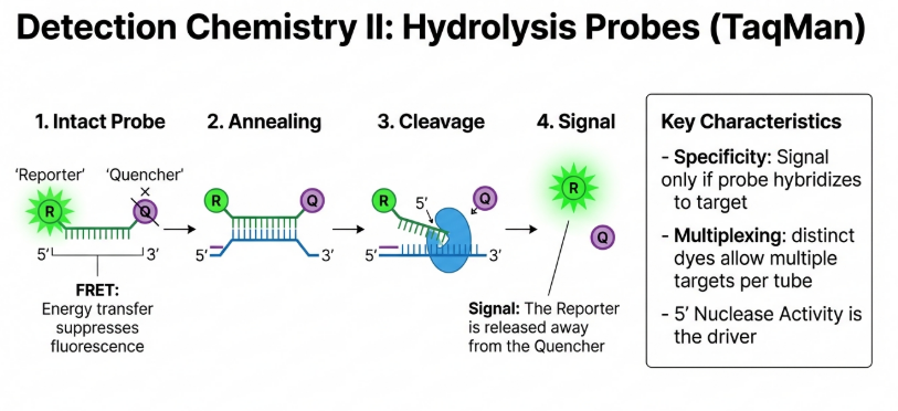
The Anatomy of a TaqMan Probe: A Silent Sentinel

The TaqMan probe is a dual-labeled fluorogenic hybridization probe. It consists of a short oligonucleotide sequence designed to bind to an internal region of the target DNA, between the two flanking primers. This “third primer” design adds an essential layer of specificity: even if the primers bind non-specifically to an unintended target, no signal is generated unless the probe also finds its exact match.

The probe’s behavior is dictated by two molecules attached to its ends:

• The Reporter (FAM): Typically 6-carboxyfluorescein, this dye emits a fluorescent signal when excited by the instrument’s light source.

• The Quencher (TAMRA): 6-carboxy-tetramethyl-rhodamine serves as the acceptor molecule.

• The Specific Sequence: A conserved genetic “fingerprint” (such as a region of the 16S rRNA gene) that ensures the assay only detects the organism of interest.

The core physics at play here is FRET (Fluorescence Resonance Energy Transfer). As long as the probe is intact, the Quencher remains in close proximity to the Reporter, absorbing its energy and releasing it as heat rather than light. Consequently, the probe remains “silent” or dark.

The 5′ Nuclease Activity: The Molecular Scissors

The biological lynchpin of the TaqMan assay is the dual functionality of Taq DNA polymerase. Beyond its role as a “builder” that incorporates nucleotides, this enzyme possesses a unique 5′ to 3′ nucleolytic activity. It acts as a pair of molecular scissors that only activate when they encounter a physical obstacle on the DNA strand.

The interaction between the polymerase and the probe occurs in a precise sequence during the extension phase:

1. Hybridize: As the reaction cools during the annealing phase, the primers and the TaqMan probe bind to their respective complementary sequences on the target DNA.

2. Extend: The temperature is raised (often to 60°C or 72°C), and Taq polymerase begins synthesizing a new DNA strand from the 3′ end of the primer.

3. Cleave: As the polymerase moves along the strand, it reaches the bound probe. Using its 5′ nuclease activity, the enzyme physically displaces and cleaves the probe into fragments.

The “Magic” of Fluorescence Release

Cleavage is the catalyst for light. Once the reporter is chopped away from the probe, it is no longer within the FRET-required distance of the quencher. This separation “releases” the fluorescence, allowing the instrument’s CCD camera to detect a signal.

Crucially, the instrument does not simply measure raw light. It performs a normalization calculation. Because the Quencher (TAMRA) signal remains relatively stable throughout the reaction, it is used as an internal standard to normalize the fluctuating Reporter (FAM) signal. The software calculates a value known as ΔRn, which is the ratio of the reporter signal to the quencher signal, minus the baseline.

There is a direct mathematical correlation between biology and light. Because exactly one probe molecule is cleaved for every new DNA strand synthesized, the increase in fluorescence is directly proportional to the amount of DNA being copied. More DNA Copies = More Probe Cleavage = Higher ΔRn Signal.

Comparative Analysis of Detection Chemistries

Feature	Non-Specific Dyes (e.g., SYBR Green)	Specific Probes (e.g., TaqMan)
Mechanism	Binds to minor groove of any dsDNA	Hybridization followed by 5′ nuclease cleavage
Specificity	Lower (detects primer-dimers)	High (only detects targeted sequence)
Multiplexing	Limited / Difficult	Excellent (using different fluorophores)
Post-PCR Requirement	Melting Curve Analysis Required	No (but may require gel verification for high CT​)

Why TaqMan is a Laboratory Gold Standard

While non-specific dyes like SYBR Green are cost-effective, they lack the diagnostic rigor of TaqMan. SYBR Green will fluoresce in the presence of any double-stranded DNA, including primer-dimers or non-specific products. TaqMan’s requirement for three independent hybridization events (two primers and one probe) ensures unmatched accuracy.

In clinical research—such as the detection of the periodontal pathogen Porphyromonas gingivalis targeting the 16S rRNA gene—the superiority of qPCR is evident. Clinical data show that while anaerobic culture may only detect the pathogen in 50% of overall samples due to the bacteria’s fastidious growth requirements, qPCR achieves an overall detection rate of 59.4%, representing 100% sensitivity relative to culture.

The TaqMan Advantage

Feature	Traditional Anaerobic Culture	TaqMan Real-Time PCR (qPCR)
Specificity	Relies on phenotypic traits and growth requirements.	Relies on a specific genetic “fingerprint” (e.g., 16S rRNA).
Throughput	Slow; requires 7–10 days of incubation.	Fast; results in hours via 96-well automation.
Sensitivity	Lower; misses non-viable or oxygen-sensitive cells.	100% Sensitivity; detects non-viable cells and single molecules.
Quantification	Measured in CFU/mL (Living colonies only).	Measured in Genome Equivalents (Total DNA load).

By harnessing the 5′ nuclease activity of Taq polymerase and the physics of FRET, the TaqMan mechanism provides the sensitivity and specificity required for the highest levels of molecular diagnostics. For the aspiring scientist, mastering this tool is a gateway to quantifying the previously invisible world of genetic information.

4. Quantification Mechanics: Ct​ Values and Normalization

 Defining the Cycle Threshold (Ct)

The most reliable metric for quantification is the Cycle Threshold (Ct) value. This value is determined by assigning an arbitrary line—the Threshold—that must be positioned within the log-linear phase of the amplification plot.

Formal Definition: The Ct value is the cycle number at which the fluorescence signal (ΔRn) generated within a reaction crosses a designated threshold. This threshold is typically set at 10 standard deviations above the mean of the base-line emission calculated from cycles 1 to 15.

The Diagnostic Superiority of the Ct Value:

• Reliability: By measuring the signal during the log-phase, we avoid the variability and “late cycle inhibition” often seen in the plateau phase, which can lead to early plateaus and misleading final intensities.

• Predictive Power: The cycle at which a sample crosses the threshold is inversely proportional to the logarithm of the initial target quantity.

• High-Throughput Accuracy: Modern instrumentation (e.g., ABI Prism 7700 or CFX96) automates this detection across 96-well formats, eliminating the labor-intensive post-PCR handling associated with gel electrophoresis.

The Inverse Relationship: DNA Quantity vs. Ct

The core mathematical principle of qPCR is the inverse linear relationship between the starting target quantity and the resulting Ct value. If a sample contains a high concentration of the target (such as the 16S rRNA gene of a pathogen), it will require fewer doubling cycles to reach the threshold, resulting in a lower Ct. Conversely, fewer starting copies require more cycles, shifting the plot to the right.

• The Linear Predictor: The relationship is expressed as Ct=k⋅log(N0​)+Ct(1), where N0​ is the initial number of template molecules.

• The Logic of the Shift: A reaction starting with fewer copies must undergo more rounds of exponential amplification to accumulate enough cleaved probe to trip the threshold sensor.

[!NOTE] The Doubling Principle and Efficiency While 100% efficiency assumes a perfect doubling per cycle (E=1), biological samples often exhibit slightly lower efficiency (e.g., E=0.90). The ratio of starting DNA between two samples (A and B) is calculated using the following efficiency-corrected formula:

Ratio = (1+E)^{(CtB​−CtA​)}

An analyst must account for this; a 4-cycle difference at 100% efficiency (E=1) represents a 16-fold difference, whereas at 90% efficiency (E=0.9), it represents only a ~13-fold difference.

Key Takeaways for Quantification

• The Ct​ Value: A lower Ct​ value indicates a higher starting concentration of target DNA. If Sample A reaches the threshold at cycle 20 and Sample B at cycle 24, Sample A contained significantly more DNA.

• Linearity: Ct​ values decrease linearly as the log of the target quantity increases.

• Dynamic Range: One of the greatest advantages of TaqMan chemistry is its massive dynamic range, which can span six orders of magnitude (approaching a 1,000,000-fold difference in starting material). This allows for the simultaneous detection of both trace amounts and high concentrations of DNA in a single run.

The Impact of PCR Efficiency (E)

Quantification accuracy is contingent upon PCR efficiency. In a perfect reaction (E=100%), the target doubles every cycle. However, biological “matrix effects” caused by inhibitors like heme, heparin, or IgG often reduce this efficiency. Consider a 4-cycle difference between samples:

• At 100% efficiency: 24=16-fold difference.

• At 90% efficiency: (1+0.9)4=13-fold difference.

From Plot to Prediction: The Standard Curve

To transition from relative comparisons to absolute quantification, the analyst constructs a Standard Curve using serial dilutions of a known template. By plotting the Ct values against the logarithm of the initial concentrations, unknown samples can be quantified through extrapolation to the x-axis.

Interpreting the Standard Curve

Metric	Definition	Impact on Result
Slope (k)	The steepness of the regression line.	Used to calculate Efficiency: E=10−1/k−1. A slope of −3.32 indicates 100% efficiency.
Intercept	The theoretical Ct value for a single target molecule.	Represents the analytical sensitivity (the lower limit of detection) of the assay.

In clinical application, these metrics are vital for assessing bacterial load. For instance, in the diagnosis of periodontitis, RT-PCR targeting the 16S rRNA gene of P. gingivalis has demonstrated 100% sensitivity and 90.6% accuracy compared to traditional anaerobic culture. These loads show a moderate positive correlation (r≈0.42) with clinical parameters like Probing Depth (PD) and Clinical Attachment Loss (CAL), providing a precise window into disease severity.

Normalization and Standard Additions

In a clinical laboratory setting, we must correct for isolation losses and matrix-driven inhibition. Normalization is achieved by measuring a reference gene (housekeeping gene) such as β-actin, which remains relatively constant across samples. For samples with significant inhibitory matrices, the method of standard additions or the use of exogenous “spikes” allows us to calculate the true initial concentration by observing how the matrix affects a known quantity of added template.

5. Reverse Transcription (RT) Strategies for Gene Expression

To analyze RNA, it must first be converted to cDNA. This step is the largest source of experimental noise; average RT yields are often only 30%, and yields can vary up to 100-fold depending on the enzyme (MMLV vs. AMV) and priming strategy.

Priming Strategies

1. Oligo(dT) / Anchored Oligo(dT): Hybridizes to the poly(A) tail. Anchored Oligo(dT) (using one or two non-thymine bases at the 3′ end) ensures the primer binds exactly at the start of the A-tail, providing more homogenous transcripts.

2. Random Hexamers / Nonamers: Preferred for degraded or archival RNA. Random Nonamers bind more strongly than hexamers, making them superior for high-temperature RT protocols designed to resolve secondary RNA structures.

3. Gene-Specific Primers: The most specific approach, often used in one-step RT-PCR formats to minimize contamination and maximize sensitivity for a single target.

6. Clinical Application: Detecting Porphyromonas gingivalis in Periodontitis

The clinical superiority of RT-PCR over anaerobic culture is demonstrated in the detection of Porphyromonas gingivalis, a “red complex” pathogen. A study by Rachita et al. utilized RT-PCR targeting the 16S rRNA gene with a TaqMan probe to evaluate diagnostic performance.

Comparative Performance

Traditional culture often underestimates fastidious pathogens due to strict growth requirements. RT-PCR identified P. gingivalis in 59.4% of samples, compared to 50% by culture. Notably, RT-PCR achieved 100% sensitivity because it detects low-abundance and non-viable cells that culture misses.

Data Insight

The study established a clear link between bacterial load and disease severity. Moderate positive correlations (r≈0.35–0.42) were observed between the P. gingivalis quantity and clinical parameters: Probing Depth (PD), Clinical Attachment Loss (CAL), and Gingival Index (GI). These metrics confirm that RT-PCR quantification is a valid proxy for disease activity.

7. Strategic Advantages and System Limitations

Advantages

• Throughput & Automation: Compatible with 96/384-well formats and liquid handling.

• Contamination Control: “Closed-tube” systems eliminate post-PCR handling, drastically reducing carry-over contamination risk.

• Dynamic Range: Accurate quantification across at least five orders of magnitude.

Limitations

• Viability Bias: Because RT-PCR detects DNA remnants, it cannot distinguish between active and non-viable infections without specialized dyes like propidium monoazide.

• Inhibitory Matrices: Clinical samples containing heme or IgG require robust extraction protocols or standard curves to prevent underquantification.

8. Conclusion: The Future of Precision Diagnostics

Real-Time PCR is the definitive gold standard for sensitive and rapid nucleic acid quantification. Moving beyond the limitations of traditional culture and endpoint PCR, it provides the precise data required for personalized medicine and risk assessment. As evidenced by its application in periodontal pathogen detection, the adoption of RT-PCR is essential for clinicians seeking superior diagnostic accuracy and targeted therapeutic outcomes.

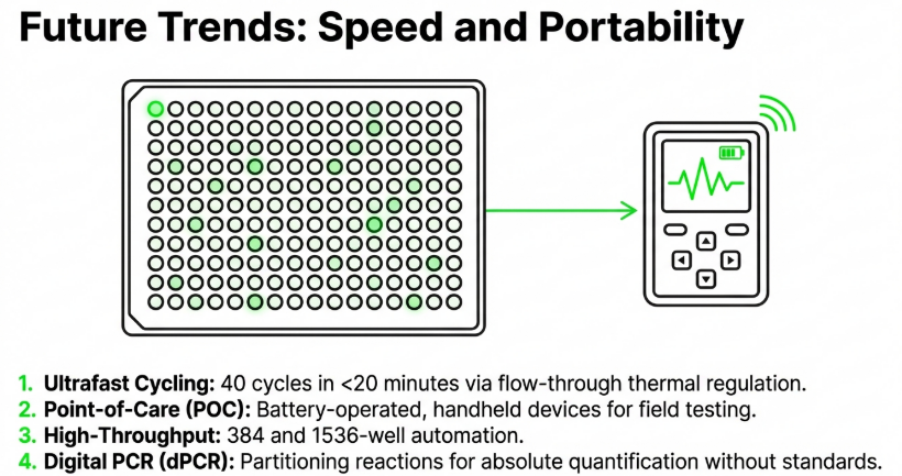
Image Summary

Questions/Answers

1. What are the core differences between absolute and relative PCR quantification?

The core differences between absolute and relative PCR quantification lie in how the data is interpreted, the type of standards used, and the final units of measurement.

1. Fundamental Definition and Result Expression

• Absolute Quantification: This method determines the exact copy number or concentration of a target nucleic acid in a sample. Results are expressed in specific units, such as copies per cell, copies per microgram of cDNA, or nanograms of DNA.

• Relative Quantification: This approach measures the relative change in expression of a target gene compared to a reference sample (calibrator) or an internal control. Instead of an exact number, results are typically expressed as a fold change or ratio (e.g., a “fivefold increase” in expression).

2. Standards and Calibration

• Absolute Quantification: It requires the construction of a standard calibration curve using serial dilutions of a standard with a known, precise concentration. Common standards include purified plasmids containing the target gene, genomic DNA, or synthetic oligonucleotides.

• Relative Quantification: It does not require a standard curve of known concentrations. Instead, it relies on an internal control gene (often a “housekeeping” gene like β-actin or GAPDH) to normalize for variations in the amount and quality of starting material between samples.

3. Effort and Complexity

• Absolute Quantification: This method is generally more labor-intensive because the researcher must precisely quantify and validate stable standards and include them in every PCR run.

• Relative Quantification: It is considered more practical for most research applications because it eliminates the need to produce and maintain accurate standards for every target gene.

4. Primary Applications

• Absolute Quantification: This is critical when a precise quantity is necessary, such as calculating viral or bacterial loads in clinical samples, determining the number of transgene integrations, or measuring GMO content in food.

• Relative Quantification: This is the preferred method for gene expression studies where the investigator wants to see how a treatment or biological state (e.g., disease vs. healthy) affects mRNA levels compared to a control.

Summary Table of Core Differences

Feature	Absolute Quantification	Relative Quantification
Goal	Exact copy number/mass	Fold change/ratio
Standards	Known external standards (e.g., plasmids)	Internal control/housekeeping genes
Calibration	Required standard curve	Not required (or uses arbitrary units)
Effort Level	High (labor-intensive)	Lower
Typical Use	Viral load, pathogen detection	Gene expression analysis

2. How do standard curves evaluate PCR amplification efficiency?

Standard curves evaluate PCR amplification efficiency by establishing a linear relationship between the logarithm of a known template concentration and the resulting quantification cycle (Cq or Ct) value. This process allows researchers to determine how closely the reaction approaches the theoretical ideal of doubling the target DNA in every cycle.

1. Construction and Plotting

To evaluate efficiency, a serial dilution of a standard (such as a plasmid, genomic DNA, or synthetic oligonucleotide) is prepared, typically using five- to ten-fold steps. The Cq values obtained from these dilutions are plotted on the y-axis against the logarithm of the initial concentration or copy number on the x-axis. A linear regression is then performed to calculate the slope of the line.

2. The Efficiency Formula

The PCR amplification efficiency (E) is mathematically derived from the slope (m) of the standard curve using the following equation: E=10−1/m−1 (expressed as a value between 0 and 1, or 0% and 100%).

Some models define efficiency as a value between 1 and 2, representing the fold-increase per cycle, using the formula E=10−1/m.

3. Interpreting the Results

• Ideal Efficiency: A slope of −3.322 corresponds to an efficiency of 100%, meaning the number of DNA molecules exactly doubles in each cycle.

• Acceptable Range: In practice, an efficiency between 90% and 110% (corresponding to slopes between −3.6 and −3.1) is generally considered acceptable for a validated assay.

• Linearity (R2): The coefficient of determination (R2) is used to assess the reliability of the standard curve. An R2 value ≥0.98 or 0.99 indicates a strong linear relationship and suggests that the amplification is consistent across the entire dynamic range.

4. Identifying Reaction Issues

The standard curve provides critical diagnostic information about the health of the PCR:

• Inhibition: If an inhibitor is present in the most concentrated samples, it will cause a visible increase in Cq values, resulting in a diminished Cq span (less than 3.322) between those dilutions.

• Pipetting Errors: High variability or scatter in Cq values at lower concentrations typically suggests pipetting errors or stochastic effects rather than chemical inhibition.

• Sensitivity: The y-intercept of the curve represents the theoretical Cq value at which a single copy of the target would be detected, helping define the assay’s analytical sensitivity.

3. What are the advantages of TaqMan versus SYBR Green?

Choosing between TaqMan (hydrolysis probes) and SYBR Green (intercalating dyes) involves weighing specificity and multiplexing capabilities against cost and versatility.

Advantages of TaqMan over SYBR Green

• Superior Specificity: TaqMan’s greatest advantage is its inherent specificity. A fluorescent signal is only generated when three separate sequences (two primers and one probe) hybridize correctly to the target. In contrast, SYBR Green binds non-specifically to all double-stranded DNA, meaning it also detects artifacts like primer-dimers and non-specific products.

• Multiplexing Capability: Because probes can be labeled with different, distinguishable reporter dyes (e.g., FAM, HEX, VIC), TaqMan allows for the simultaneous detection of multiple targets in a single reaction tube. SYBR Green generally does not support multiplexing because it cannot distinguish between different amplicons in the same way.

• Data Convenience: TaqMan data is often considered more reliable and simpler to work with because no post-PCR analysis (like melt curves) is required to confirm that the correct target was amplified.

• Allelic Discrimination: TaqMan is ideal for identifying single-nucleotide polymorphisms (SNPs) and point mutations, which are difficult to distinguish with SYBR Green.

• Rare Target Detection: Probes are recommended for rare targets (quantification cycles/Cq > 30) where the potential for non-specific interference is higher.

Advantages of SYBR Green over TaqMan

• Cost-Effectiveness: SYBR Green is significantly less expensive because it does not require the design and synthesis of a specialized, fluorescently labeled probe for every gene being studied.

• Versatility and Flexibility: The same SYBR Green dye can be used with any pair of primers for any target. This makes it much easier to apply to already established PCR assays without a second design stage.

• Initial Optimization: SYBR Green is often preferred for early experimental stages and screening many different genes due to its lower upfront cost and simpler assay design.

• Potential for High Precision: Some studies have reported that SYBR Green can be more precise, yielding lower coefficients of variation and more linear decay plots than TaqMan assays in certain contexts.

Summary Comparison Table

Feature	TaqMan (Hydrolysis Probes)	SYBR Green (Intercalating Dyes)
Specificity	Very High (requires probe binding)	Lower (binds all dsDNA)
Multiplexing	Yes (different colors)	Generally No
Cost	High (expensive probes)	Low (inexpensive dye)
Ease of Use	Harder (requires probe design)	Easier (uses existing primers)
Confirmation	Not required	Requires melting curve analysis
Target Abundance	Recommended for rare targets	Sufficient for abundant targets

4. How does PCR inhibition impact diagnostic sensitivity and accuracy?

PCR inhibition significantly compromises diagnostic sensitivity and accuracy by interfering with the biochemical processes of the reaction, often leading to the underestimation of target quantities or entirely failing to detect a pathogen.

1. Impact on Diagnostic Sensitivity

Inhibitory substances reduce sensitivity by increasing the Limit of Detection (LOD), meaning a higher concentration of the target is required for a positive result.

• False Negatives: The most critical impact on sensitivity is the production of false-negative results. This occurs when inhibitors prevent the reaction from reaching the detection threshold, even if the target pathogen is present.

• Target Concentration Effects: Sensitivity is particularly affected in samples with low numbers of target cells (e.g., early-stage infections or environmental samples), where even mild inhibition can prevent any detectable amplification.

• Matrix Specificity: Certain matrices are notoriously inhibitory; for instance, complex samples like feces, stool, or sputum are more likely to compromise sensitivity than cleaner matrices like serum or plasma.

2. Impact on Diagnostic Accuracy

Accuracy—the level of agreement between measured and true values—is degraded through the diminishment of PCR efficiency and the distortion of data interpretation.

• Underestimation of Quantities: Inhibitors can cause a sample to exhibit a higher threshold cycle (Ct) value than it would in an uninhibited state. Because Ct values are predictive of initial target quantity, this results in the underestimation of the true number of microorganisms or the viral/bacterial load.

• Efficiency Variations: PCR quantification assumes that efficiency is constant and ideally close to 100%. Inhibitors (like calcium or hematin) lower this efficiency, and even a small 10% difference in efficiency can result in huge data distortion and “wrong” quantification results.

• Unreliable Data Interpretation: If calculations are not adjusted for the presence of inhibitors, the resulting interpretations can be severely skewed, making it impossible to accurately compare results between different samples or across different runs.

3. Mechanisms of Inhibition Affecting Results

The physical ways inhibitors act directly determine how sensitivity and accuracy are lost:

• Taq Polymerase Interference: Substances like calcium, hematin, and tannic acid can bind to or deactivate the DNA polymerase, reducing reaction efficiency and final product concentration.

• DNA Template Binding: Inhibitors such as humic acid and melanin bind to the DNA template itself, limiting its availability for the polymerase and shifting the Ct cycle higher.

• Fluorescence Interference: Some inhibitors (e.g., collagen or indigo) can quench the fluorescent signal or increase background noise, interfering with the instrument’s ability to accurately monitor the reaction in real time.

To mitigate these impacts, diagnostic assays often incorporate internal amplification controls (IC) to detect inhibition and validate negative results. If an internal control fails to amplify, the diagnostic result is considered unreliable because of the presence of inhibitors.

5. Can standard curves be used for relative quantification too?

Yes, standard curves can be used for relative quantification, and they are considered a reliable and simple alternative to methods based on PCR efficiency assessment (such as the 2−ΔΔCq method). While standard curves are the primary tool for absolute quantification, there are “no barriers” to employing them for relative studies.

How Standard Curves Work for Relative Quantification

In relative quantification, the standard curve does not require known absolute concentrations (like copies/μl). Instead:

• Arbitrary Units: The curve is constructed using a serial dilution of a calibrator sample (a reference material, such as a pool of all cDNA samples), and concentrations are expressed in arbitrary units or relative dilution factors.

• Interpolation: The Cq values of unknown samples are interpolated into this relative standard curve to determine an initial “quantity” for the target gene.

• Normalization: These values are then normalized to the quantity of an internal reference gene (housekeeping gene) obtained from its own relative standard curve.

Advantages of the Standard Curve Method

• Reliability and Simplicity: It simplifies the data processing and avoids theoretical and practical problems associated with precisely assessing PCR efficiency for every individual sample.

• Validation: Including a standard curve on each PCR plate provides routine validation for the methodology of that specific run.

• Flexibility: It can be used even when the amplification efficiencies of the target and reference genes are unequal, which is a situation where the simpler 2−ΔΔCq method would generate errors.

Disadvantages and Trade-offs

• Labor and Cost: The main drawback is the increased effort and cost required to prepare, validate, and run standard curves on every plate.

• Capacity: Because standard curves occupy several wells (e.g., a 6-point curve in triplicates takes 18 wells), they reduce the number of experimental samples that can be analyzed in a single run.

In summary, for research where reliability of results is prioritized over costs and labor load, the standard curve approach is a preferred alternative for processing relative real-time PCR data.

6. How do standard curves determine the limit of detection?

Standard curves determine the limit of detection (LOD) by establishing the lower boundary of an assay’s linear dynamic range and providing the mathematical parameters needed to calculate the minimum detectable amount of a target.

Here is how standard curves are used to determine the LOD:

1. Determining Theoretical Sensitivity via the Y-Intercept

In a standard curve regression equation (y=mx+c), the y-intercept (c) represents the theoretical quantification cycle (Cq or Ct) value at which a single copy of the target DNA would be detected. While this is a theoretical value, it provides a baseline for the absolute maximum sensitivity of the PCR assay.

2. Defining the Linear Dynamic Range

The LOD is closely tied to the assay’s dynamic range, which is the range over which the reaction is linear.

• Linearity (R2): A standard curve must maintain a coefficient of determination (R2) ≥0.98 to be considered reliable.

• Lower Bound: The LOD is typically determined experimentally as the lowest concentration within this linear range that still yields a fluorescent signal significantly different from negative controls.

3. Experimental Validation with Replicates

Because low-concentration samples are subject to stochastic (random) effects, the LOD is defined through the analysis of multiple replicates at the lower end of the standard curve.

• The 95% Rule: In practice, the LOD is often defined as the lowest concentration on the standard curve where at least 95% of the replicates produce a positive amplification signal.

• Confidence Levels: Testing more replicates (typically 6 to 15 or more) allows for a narrower interval of confidence and a more precise determination of the LOD.

4. Mathematical Calculation (ICH Guidelines)

For some assays, the LOD is calculated mathematically using the slope (m) of the standard curve and the standard deviation of the response (sd) according to the following formula: LOD=3.3×sd/m.

5. Statistical Modeling (Probit/Logit)

Researchers may use the data from the standard curve to perform Probit or Logit regression analysis. These mathematical functions transform the sigmoid dose-response curve into a straight line, allowing them to calculate the exact concentration coupled with a specific probability (e.g., 95%) of detection.

Important Considerations

• Theoretical vs. Practical Limits: According to the Poisson distribution, the theoretical LOD for PCR cannot be lower than three copies of the target. Any experimental LOD lower than this is considered statistically meaningless.

• Whole-Method LOD: In diagnostics, the LOD must reflect the entire process, including nucleic acid isolation and recovery efficiency, rather than just the PCR step alone.

• Cq Values Below LOD: Samples yielding Cq values below the determined LOD are still valid indicators of a microorganism’s presence; however, the probability of repeated detection at that level is lower than 95%.

7. What causes a reaction to exceed 100% efficiency?

In theoretical PCR amplification, the maximum efficiency is 100%, meaning the amount of target DNA exactly doubles with every cycle. However, in practice, researchers often observe calculated efficiencies exceeding 100% (sometimes reported up to 110% or 120%), which is generally attributed to experimental artifacts or mathematical overestimation rather than a physical reality.

The primary causes for a reaction appearing to exceed 100% efficiency include:

1. Inhibition in Concentrated Standards

The most common cause for calculated efficiency >100% is the presence of inhibitors in the most concentrated samples of a standard curve. Inhibitors can increase the quantification cycle (Cq) values for these high-concentration samples, making them appear to have less DNA than they actually do. This results in a diminished Cq span (less than the ideal 3.322 cycles between ten-fold dilutions). Mathematically, a shallower slope (e.g., closer to –3.0 than –3.32) results in a calculated efficiency greater than 100%.

2. Methodological Overestimation

The standard method of calculating efficiency from the slope of a calibration curve (E=10−1/slope−1) is prone to overestimation. Because this calculation relies on a simple linear approximation of data across several dilutions, it does not account for the PCR efficiencies in individual target samples, which may vary. Sources note that while this method is highly reproducible, it often yields results where E>2.0 (100%), indicating the calculation itself is not always optimal for reflecting “real efficiency”.

3. Nonspecific Amplification

The accumulation of nonspecific products or primer-dimers can artificially inflate the fluorescent signal, especially when using intercalating dyes like SYBR Green. These artifacts compete for reaction resources and contribute to the total fluorescence recorded by the instrument. If these artifacts are present in a way that shifts Cq values non-linearly across a dilution series, they can distort the slope of the standard curve and lead to an erroneous quantification indicating excessive efficiency.

4. Technical and Instrumental Errors

Several minor technical factors can cumulatively result in a slope that appears too shallow:

• Pipetting Errors: Imprecise pipetting, particularly during the preparation of serial dilutions, can result in inaccurate template concentrations that skew the resulting standard curve.

• Baseline and Threshold Settings: If the fluorescence baseline is set incorrectly or the threshold intersects the amplification curve outside the true exponential phase, the resulting Cq values will be inaccurate, potentially leading to a distorted efficiency calculation.

• Temperature Inhomogeneity: Small local temperature deviations within the thermal cycler can lead to substantial errors in quantification across different wells, affecting the slope of the standard curve.

Summary of Acceptable Ranges

While 100% is the theoretical ideal, many diagnostic guidelines consider a range of 90% to 110% (corresponding to slopes between –3.6 and –3.1) to be acceptable for a validated assay. For qualitative multiplex tests, some guidelines even allow a broader range of 80% to 120%.

8. Why are housekeeping genes used for relative normalization?

Housekeeping genes (also referred to as internal reference genes or endogenous controls) are used for relative normalization in qPCR to minimize errors and correct for variation between samples.

The core reasons for using them include:

1. Correcting Technical and Sample-to-Sample Variation

In real-time PCR experiments, errors are introduced due to minor discrepancies in:

• Starting amount of material: Variations in the mass of tissue, cell number, or volume of sample used.

• Nucleic acid quality: Differences in RNA integrity and purity between samples.

• Enzymatic efficiency: Variations in the efficiency of the reverse transcription (cDNA synthesis) and the PCR amplification itself.

By simultaneously amplifying a target gene and a housekeeping gene, researchers can use the housekeeping gene as a denominator to cancel out these technical variations, leaving only the true biological changes.

2. Theoretical Constant Expression

Housekeeping genes are selected because they are theoretically expressed at a constant level across different tissues of an organism and at all stages of development. Because they are necessary for basic cell survival—such as β-actin (cytoskeletal protein) or GAPDH (glycolytic enzyme)—their expression is expected to remain relatively stable even under different experimental conditions.

3. Practicality and Simplification

Using housekeeping genes for relative quantification is often less labor-intensive than absolute quantification because:

• It does not require the construction of a standard calibration curve with known copy numbers for every gene being studied.

• The results can be expressed simply as a fold change (e.g., using the 2−ΔΔCq method), which is sufficient for most physiological and pathological studies comparing a treated sample to a control.

4. Important Considerations and Limitations

While housekeeping genes are the “gold standard” for normalization, sources emphasize several caveats:

• No gene is perfectly stable: Many common housekeeping genes like GAPDH and β-actin have been shown to fluctuate under certain treatments or biological states (e.g., disease vs. healthy).

• Validation is required: The stability of a chosen reference gene must be validated for the specific experimental conditions before use.

• Multiple reference genes: To improve accuracy, modern guidelines (like MIQE) often recommend using the geometric mean of three or more validated reference genes for normalization rather than relying on a single one.

9. What is the ‘MIQE’ guideline for standardizing PCR?

The MIQE guidelines, which stand for “Minimum Information for Publication of Quantitative Real-Time PCR Experiments,” were established in 2009 to promote consistency between laboratories, increase experimental transparency, and ensure the integrity of scientific literature.

The primary goal of the MIQE guidelines is to address a lack of consensus on how to perform and interpret qPCR experiments, ensuring that publications provide enough detail for readers to critically evaluate the quality of the results or repeat the experiments.

Core Components of MIQE

The guidelines provide a comprehensive checklist that researchers are encouraged to submit alongside their manuscripts. This checklist covers nine major components of a qPCR experiment:

1. Experimental design: The overall setup and logic of the study.

2. Sample: Information about the biological source and handling.

3. Nucleic acid extraction: Details on how DNA or RNA was isolated and its quality assessed.

4. Reverse transcription: Parameters for converting RNA to cDNA (critical for RT-qPCR).

5. qPCR target information: Sequences and characteristics of the genes being studied.

6. qPCR oligonucleotides: Precise details on primer and probe sequences.

7. qPCR protocol: Specific cycling conditions, reagents, and instruments used.

8. qPCR validation: Evidence of the assay’s performance, including efficiency and specificity.

9. Data analysis: The mathematical models and statistical tests applied to the raw data.

Key Standardization Requirements

• Terminology (Cq): MIQE standardized the term quantification cycle (Cq) to replace various manufacturer-specific terms like Ct, Cp, or TOP.

• Reference Gene Validation: The guidelines emphasize that using a single, non-validated reference gene is unacceptable. Instead, they recommend using the geometric mean of three or more validated reference genes for accurate normalization.

• Dynamic Range: MIQE defines the dynamic range as the span over which a reaction is linear, recommending that it should cover at least 3 orders of magnitude and ideally extend to 5 to 6 log10 concentrations.

• Transparency: Reviewers use MIQE to assess the validity of protocols through the full disclosure of all reagents, sequences, and analysis methods.

Related Guidelines

Following the success of MIQE, the dMIQE guidelines were introduced to provide similar standardization for digital PCR (dPCR) experiments. Additionally, while MIQE focuses on quantitative assays, similar template tables have been developed for qualitative qPCR to help reviewers evaluate the validity of those assays for publication.

10. How do matrix effects influence the limit of detection?

Matrix effects significantly influence the limit of detection (LOD) in PCR by introducing inhibitory substances and reducing the efficiency of nucleic acid recovery, which together can drastically lower the assay’s sensitivity. Because complex samples often contain substances that interfere with the reaction, the LOD for a target organism in a clinical or environmental matrix is typically much higher (less sensitive) than its theoretical LOD in pure water.

1. Mechanisms of Matrix Interference

Matrix effects alter the LOD through two primary pathways:

• Reduction in DNA Recovery: Complex matrices like food, feces, and soil make it difficult to extract and purify target DNA. The efficiency of DNA recovery from these samples is often 30% or lower; neglecting this parameter leads to an underestimation of the target concentration and an inaccurate (lower) LOD value for the overall method.

• PCR Inhibition: Inhibitors co-extracted from the matrix can interfere with the biochemical process of PCR. They may bind to the DNA polymerase (e.g., calcium, hematin), bind to the DNA template (e.g., humic acid, melanin), or quench the fluorescent signal (e.g., collagen, indigo). These interactions reduce amplification efficiency, requiring a higher initial target concentration to reach the detection threshold.

2. Comparative Impact of Different Matrices

The influence on LOD varies dramatically depending on the specific sample type:

• High Sensitivity Matrices: Spiked water samples typically exhibit the lowest (best) LOD because they have a low presence of inhibitors.

• Highly Inhibitory Matrices: Milk samples often demonstrate the highest (worst) LOD values due to interference from high levels of fat, protein, and calcium. For example, studies on Brucella detection show a significantly higher mean LOD in milk (883.0 fg) compared to blood (427.6 fg).

• Significant Detection Drops: In diagnostic applications for plant pathogens, targets that could be detected at 100 CFU/mL in pure culture saw detection thresholds drop to 105 or 106 CFU/mL when tested in potato tuber extracts due to severe matrix inhibition.

3. Impact on Diagnostic Reliability

Matrix effects can lead to false-negative results, particularly when target cells are expected in low numbers. If inhibitors prevent the reaction from reaching the detection threshold, the assay will fail even if the pathogen is present. Consequently, a diagnostic result is considered unreliable if inhibitors are detected (e.g., through an internal amplification control) and not removed.

4. Requirement for Matrix-Specific Validation

Because of these induced effects, a material-specific validation approach is essential. In practice, the LOD is determined by spiking multiple aliquots of a specific matrix (e.g., milk, stool, or sputum) with serial dilutions of the target organism to undergo the entire process of isolation and qPCR. The LOD is then experimentally defined as the lowest concentration that can be detected in 95% of the replicates within that specific matrix.

To mitigate these effects, researchers often use techniques like pre-enrichment in culture media (to dilute inhibitors and multiply target cells) or specialized extraction procedures (such as immunomagnetic separation) to generate PCR-compatible samples from heterogeneous biological material.

References

Artika, I. M., Dewi, Y. P., Nainggolan, I. M., Siregar, J. E., & Antonjaya, U. (2022). Real-Time Polymerase Chain Reaction: Current Techniques, Applications, and Role in COVID-19 Diagnosis. In Genes (Vol. 13, Number 12). MDPI. https://doi.org/10.3390/genes13122387
Ding, R., Zhang, J., & Chen, C. (2025). The thermal cycling methods for rapid PCR. In Critical Reviews in Biotechnology. Taylor and Francis Ltd. https://doi.org/10.1080/07388551.2025.2540368
Espy, M. J., Uhl, J. R., Sloan, L. M., Buckwalter, S. P., Jones, M. F., Vetter, E. A., Yao, J. D. C., Wengenack, N. L., Rosenblatt, J. E., Cockerill, F. R., & Smith, T. F. (2006). Real-time PCR in clinical microbiology: Applications for routine laboratory testing. In Clinical Microbiology Reviews (Vol. 19, Number 1, pp. 165–256). https://doi.org/10.1128/CMR.19.1.165-256.2006
Fraga, D., Meulia, T., & Fenster, S. (2014). Real-Time PCR. Current Protocols in Essential Laboratory Techniques, 2014, 10.3.1-10.3.40. https://doi.org/10.1002/9780470089941.et1003s08
Houghton, S. G., & Cockerill, F. R. (2006). Real-time PCR: Overview and applications. In Surgery (Vol. 139, Number 1, pp. 1–5). https://doi.org/10.1016/j.surg.2005.02.010
Kralik, P., & Ricchi, M. (2017). A basic guide to real-time PCR in microbial diagnostics: Definitions, parameters, and everything. In Frontiers in Microbiology (Vol. 8, Number FEB). Frontiers Research Foundation. https://doi.org/10.3389/fmicb.2017.00108
Kubista, M., Andrade, J. M., Bengtsson, M., Forootan, A., Jonák, J., Lind, K., Sindelka, R., Sjöback, R., Sjögreen, B., Strömbom, L., Ståhlberg, A., & Zoric, N. (2006). The real-time polymerase chain reaction. In Molecular Aspects of Medicine (Vol. 27, Numbers 2–3, pp. 95–125). https://doi.org/10.1016/j.mam.2005.12.007
Mangold, K. A., Manson, R. U., Koay, E. S. C., Stephens, L., Regner, M. A., Thomson, R. B., Peterson, L. R., & Kaul, K. L. (2005). Real-time PCR for detection and identification of Plasmodium spp. Journal of Clinical Microbiology, 43(5), 2435–2440. https://doi.org/10.1128/JCM.43.5.2435-2440.2005
Rebrikov, D. V., & Trofimov, D. Y. (2006). Real-time PCR: A review of approaches to data analysis. In Applied Biochemistry and Microbiology (Vol. 42, Number 5, pp. 455–463). https://doi.org/10.1134/S0003683806050024
Valasek, M. A., & Repa, J. J. (2005). Staying Current: Technology The power of real-time PCR. Adv Physiol Educ, 29, 151–159. https://doi.org/10.1152/advan