Single Nucleotide Polymorphism (SNP) Markers: The Genomic Foundation of Modern Precision Plant Breeding

1. Introduction to the SNP Era in Plant Science

The transition from traditional phenotypic selection to marker-assisted breeding (MAB) represents a sophisticated paradigm shift in agricultural biotechnology. For decades, the reliance on visible traits—subject to significant environmental variance—limited the rate of genetic gain. The advent of molecular markers allowed for the direct interrogation of the genome; however, earlier marker systems lacked the requisite resolution and scalability for 21st-century precision breeding. Single Nucleotide Polymorphisms (SNPs) have emerged as the “gold standard” due to their ubiquity and high density across the genome, facilitating the transition to high-throughput genomic selection and fine-mapping.

The Evolution of the Genetic Toolkit

Molecular markers have evolved through three distinct generations. Each leap has been defined by an increase in throughput and a decrease in manual labor, moving us toward a fully digital understanding of the genome.

Generation	Representative Marker Type	The “So What?” (Breeder Perspective)
1st: Hybridization-based	RFLP (Restriction Fragment Length Polymorphism)	Reliable but labor-intensive. Required Southern blotting and large DNA quantities; impossible to automate for modern large-scale breeding.
2nd: PCR-based	SSR (Simple Sequence Repeats / Microsatellites)	Highly polymorphic standard. Easy to detect and codominant, but lacked the genome-wide density required for high-resolution mapping.
3rd: Sequence-based	SNP (Single Nucleotide Polymorphism)	High-throughput automation. Abundant across the genome and easily read by computers as digital data (0s and 1s), allowing for massive scalability.

Technically, SNPs are single-base pair positions in genomic DNA where different sequence alternatives, or alleles, exist among individuals. To be formally distinguished from rare mutations, the least frequent allele must maintain an abundance threshold of 1% or greater. This high frequency of allelic variation makes SNPs the most abundant form of molecular markers, offering a level of genomic diversity analysis that enables the dissection of complex, polygenic traits. As sequencing costs continue to decline, the strategic deployment of SNP-based technologies is essential for accelerating the development of resilient, high-yielding crop varieties.

SNP Classification and Breeding Utility

SNP Category	Definition	Polymorphism Frequency	Recommended Mapping Application
Simple SNPs	Allelic differences within a single subgenome.	10–30%	General diversity and high-density linkage mapping.
Hemi-SNPs	Variation appearing homo- vs. heterozygous between individuals.	30–60%	Preferred for structured populations (F2, RIL, DH).
Homoeo-SNPs	Fixed differences between subgenomes (A vs. D).	Fixed / Monomorphic	Genomic structure analysis; not for trait mapping.

Anatomy of a SNP: Understanding the Genetic Variation

A SNP (pronounced “snip”) is a variation at a single nucleotide position in a DNA sequence. In a population, if at least 1% of individuals carry a different “letter” at a specific site, we call it a SNP.

The Molecular Mechanics

• Transitions vs. Transversions: There are two types of substitutions. A Transition swaps a purine for a purine (A↔G) or a pyrimidine for a pyrimidine (C↔T). A Transversion swaps a purine for a pyrimidine. While transversions are theoretically more possible, transitions are 1.5–2.5 times more frequent in nature due to the spontaneous deamination of 5-methylcytosine.

• Biallelic Nature: Although four nucleotides exist, SNPs are almost always biallelic (having only two versions). This “either/or” status makes them the perfect “digital” marker, easily processed by automated systems as binary code.

The “Neighborhoods” of DNA

The functional effect of a SNP is determined by where it resides in the genome:

• cSNP (Coding SNP): Located in exons. These can be synonymous (no change to protein) or non-synonymous (altering protein function).

• iSNP (Intronic SNP): Located in the non-coding introns. These can sometimes affect gene splicing.

• rSNP (Regulatory SNP): Located in regulatory regions. These act as the “control center” for gene expression.

• pSNP (Promoter SNP): A specific type of rSNP located in the promoter region, often influencing the “volume” of protein production.

2. Strategic Justification: The Transition from Legacy Markers to Scalable SNP Platforms

The transition from legacy PCR-based markers to Single Nucleotide Polymorphism (SNP) platforms is not merely a technical upgrade; it is an operational imperative for commercial breeding programs. Conventional breeding in perennial species like oil palm (Elaeis guineensis) is fundamentally hindered by its “temporally dioecious” nature—alternating male and female inflorescences—and extremely long life cycles. To overcome the limitations of land, energy, and environmental stress, organizations must prioritize the shift from labor-intensive sampling to automated, data-rich precision breeding. This evolution is categorized into three distinct evolutionary classes: Class 1 (Hybridization-based), Class 2 (PCR-based), and Class 3 (DNA Chip and Sequencing-based).

The following table differentiates the strategic value of these marker generations:

Dimension	Hybridization (Class 1)	PCR-based (Class 2)	Chip/Seq (Class 3)
Throughput Capacity	Low	Medium	High to Ultra-High
Automation Potential	Minimal (Labor-intensive)	Moderate	Full Automation Potential
Genomic Abundance	Low	Moderate	Highest (1 per 540 bp in wheat; 70 per 100kb in oil palm)
Cost-per-Data-Point	High	Moderate	Lowest

The Biallelic Advantage

The strategic driver for high-throughput adoption is the biallelic nature of SNPs. While multiallelic markers like SSRs offer higher polymorphism per locus, they are computationally cumbersome. SNPs typically exist in only two variants, facilitating a “digital” data format that is the key driver for automation and large-scale data analysis. This simplicity allows for the simultaneous analysis of millions of data points, providing the resolution necessary to bypass traditional phenotyping bottlenecks.

3. Strategic Discovery Methodologies for SNP Identification

Finding an SNP is a “needle in a haystack” challenge. In common wheat, for example, the genome is five times larger than a human’s, with a density of roughly 1 SNP per 370–540 base pairs (bp). Selecting an SNP discovery methodology requires a strategic assessment of genome complexity. While discovery is straightforward in model organisms, many critical crops have large, repeat-rich genomes that require sophisticated complexity-reduction techniques.

• In Silico Mining: This involves the computational extraction of SNPs by aligning overlapping Expressed Sequence Tag (EST) databases or genomic sequences. In polyploid species, this requires bioinformatic sophistication; for instance, researchers use PHRAP software for statistical analysis to distinguish true SNPs from homoeologous sequence variants (HSVs) without the need for initial amplification.

• Complexity Reduction (SLAF-seq, GBS, and RAD-seq): Strategies like Single Locus Amplified Fragment sequencing (SLAF-seq) and Genotyping-by-Sequencing (GBS) use restriction enzymes to target reduced portions of the genome. SLAF-seq is recognized as a “fast, accurate, highly efficient, and cost-effective method for developing large-scale SNP and InDel markers.” Other methods include RAD-seq and DArT-seq, the latter of which provides significant commercial support for breeding programs.

• Reduced Representation Shotgun (RRS): Originally designed for human genome mapping to ensure uniform marker distribution, RRS remains problematic for plant genomics. Its application is hindered by the massive, repetitive nature of genomes like wheat (16 x 10⁹ bp), which complicates the alignment of shotgun fragments.

• Conversion Strategies: To maintain continuity with historical data, breeders often convert older markers (RFLP, CAPS, RAPD) into SNPs. This targeted approach is vital for tagging high-value agronomic genes identified in earlier studies.

4. Navigating Genomic Complexity: Classification and Polyploidy

In allopolyploid crops such as wheat (hexaploid) or cotton (tetraploid), distinguishing between allelic variation (SNPs) and differences between subgenomes (HSVs) is critical for mapping accuracy.

Structural and Functional Categories:

• cSNPs / eSNPs: Found in coding/exon regions; can be synonymous or non-synonymous.

• rSNPs: Regulatory SNPs in promoter or intron regions that influence gene expression.

• Anonymous SNPs: SNPs where the functional effect is currently unknown.

Polyploid Specialization and Frequency: For allopolyploids, the value of a marker is determined by its segregation pattern:

1. Simple SNPs (10–30% of polymorphic loci): Identify allelic differences at a single subgenome; these segregate as diploid markers.

2. Hemi-SNPs (30–60% of polymorphic loci): These reveal variations that appear homozygous in one individual but heterozygous in another. They are strategically valuable in F2, RIL, and DH populations, where they allow for the detection of homozygous versus heterozygous variations.

3. Homoeo-SNPs: Differences across homoeologous subgenomes. These are often monomorphic within a species and are generally less useful for linkage mapping.

5. Technical Evaluation of High-Throughput Genotyping Platforms

Genotyping platform selection is a strategic decision based on the required marker density (Tier 1 vs. Tier 2) and the urgency of the breeding cycle.

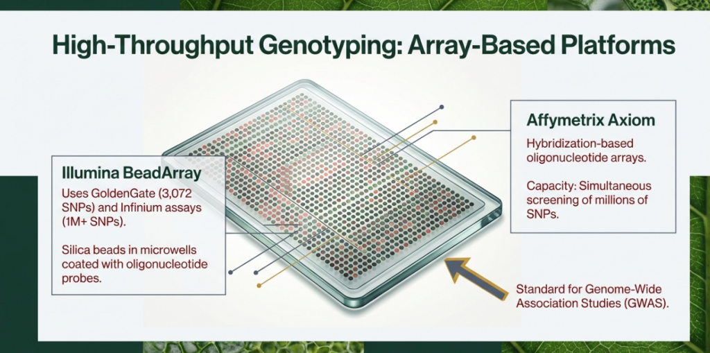
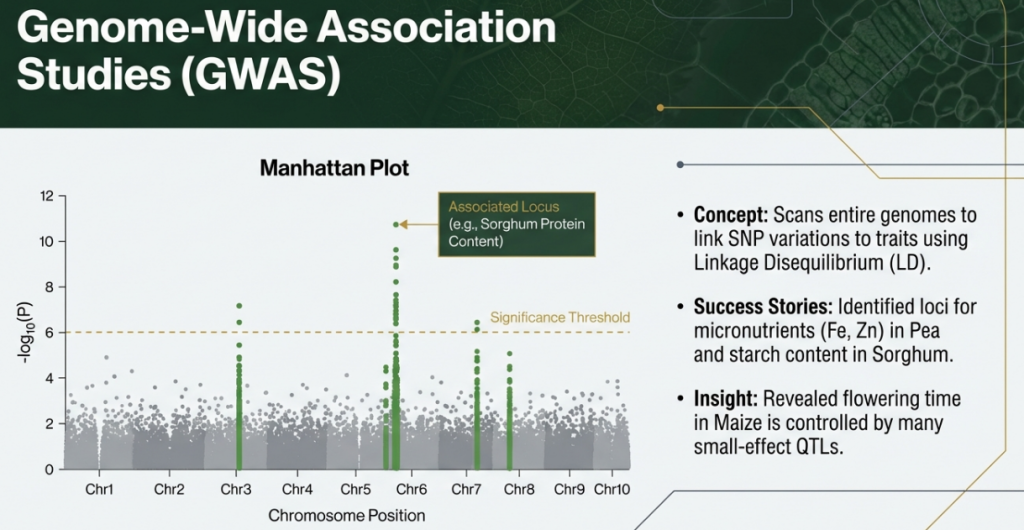
• Tier 1: Genome-Wide Discovery & GWAS

    ◦ Illumina BeadArray (GoldenGate/Infinium): Ultra-high-throughput. GoldenGate handles up to 3,072 SNPs, while Infinium arrays scale to 1.1 million. These platforms have a longer strategic lead time of 6 to 9 weeks.

    ◦ Affymetrix Axiom: Capable of handling high-density arrays, such as the 384 x 55K format, providing massive parallelization for discovery.

• Tier 2: Targeted Selection & MAS

    ◦ KASP (Kompetitive Allele-Specific PCR): A single-plex, FRET-based assay favored for flexibility. It is highly scalable, capable of achieving 150,000 data points per day, making it the primary tool for routine population screening.

    ◦ TaqMan (OpenArray): Utilizes miniaturized plates for high-sensitivity detection. It offers a rapid strategic turnaround with a 2-week lead time, making it ideal for urgent breeding decisions.

    ◦ High-Resolution Melting (HRM): A closed-tube, post-PCR format that identifies variations based on DNA melting profiles. While cost-effective for exploratory diagnostics, it is sensitive to environmental and pipetting inconsistencies.

Comparative Analysis of Genotyping Platforms

Platform	Chemistry	Technical Specification	Strategic Role
KASP	Fluorescence, single-plex	Scalable up to 150K points/day	Cost-effective for targeted gene selection (Tier 2).
TaqMan (OpenArray)	Endpoint PCR	3,072 assays per plate	High-throughput for medium-density screening.
BeadArray (Infinium)	Silica-bead microarray	XT: 96 x 50K; HD/HTS: 24 x 90K to 700K	Ultra-high-density mapping and GS (Tier 1).
GBS / DArT-seq	NGS multiplexing	Sample dependent	Discovery and genotyping for orphan crops.

Platform Decision Matrix

Breeding Scenario	Recommended Platform	Justification
Fine-mapping a resistance gene	KASP	Single-plex flexibility and low design lead time for large sample volumes.
Genome-wide background selection	BeadArray or GBS	High marker density required for rapid recurrent parent genome recovery.
Orphan/Low-resource Crop Improvement	GBS / DArT-seq	Simultaneous discovery and genotyping without prior reference genomes.

6. Implementation Stages: From Marker Validation to Practical Application

Transforming raw discovery data into a functional “Breeding Chip” requires a systematic pipeline. In oil palm, discovery efforts using tools like GATK and SAMtools have identified up to 1,261,501 reliable SNPs (MAF > 0.05), providing the library needed for elite assay development.

The Validation Workflow

1. Detection & Filtering: Filtering based on Minor Allele Frequency (MAF > 0.05) and high confidence calls.

2. Mendelian Validation: Testing in segregating populations (F2, RIL, DH) to confirm inheritance and discriminative power.

3. Final Selection: Selection of a representative subset for customized targeted assays or low-density arrays.

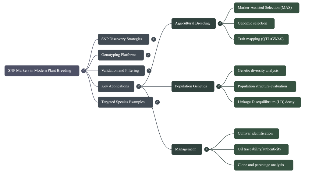
Practical Breeding Applications

1. High-Density Linkage Mapping: Saturating genetic maps to determine precise marker order, essential for positional cloning.

2. Genome-Wide Association Studies (GWAS): Identifying markers linked to complex traits, such as disease resistance (e.g., CMD in cassava) and nutritional content (e.g., carotenoids and dry matter).

3. Marker-Assisted Backcrossing (MABC): Accelerating the introgression of target traits while using background selection to maintain elite genomic integrity.

4. Haplotype Block Analysis: Evaluating linkage disequilibrium (LD) decay to refine selection accuracy. For example, the 14.5 kb average LD decay in oil palm dictates the required marker density for effective mapping.

• Linkage Disequilibrium (LD) Analysis: LD decay in oil palm is approximately 14.5 kb (ranging from 3.3 kb on Chr 15 to 19.9 kb on Chr 7). This rapid decay necessitates high-resolution arrays to prevent markers from losing association with target QTLs.

• Bioinformatics Integration: Implementation of imputation tools such as BEAGLE, IMPUTE2, or self-organizing maps is mandatory to resolve missing data in high-throughput NGS runs.

7. Operational Roadmap: Milestone-Based Integration Plan

The workflow must shift from a phenotyping-heavy mindset to a genomics-integrated pipeline to realize high genetic gain.

Phased Implementation Timeline

• Phase I: Resource Development (Months 1-6): Germplasm collection, SLAF-seq discovery, and in silico restriction enzyme digestion (HaeIII + Hpy166II) for alignment.

• Phase II: Assay Validation (Months 7-12): Designing allele-specific assays (KASP/TaqMan) and constructing high-density linkage maps across diverse panels.

• Phase III: Routine Integration (Month 13+): Deployment of Tier 1 (GWAS/GS) and Tier 2 (MABC/MAS) applications into active breeding cycles.

Strategic Outlook

The ROI of SNP integration is realized through the radical compression of breeding cycles and the ability to select for complex, polygenic traits (e.g., carotenoids, starch composition) that are traditionally difficult to phenotype. By bypassing the limitations of land and environmental stress, SNP-enabled precision breeding ensures the rapid delivery of high-yielding, resilient varieties in a data-driven commercial environment.

8. Case Studies in Genomic Application: Oil Palm and Wheat

The practical application of these technologies illustrates how SNP data translates into breeding outcomes.

Oil Palm (Elaeis guineensis): Using SLAF-seq, researchers identified 1.2 million SNPs, revealing an average SNP density of 70 SNPs/100 kb and an average physical distance between markers of 0.5 kb.

• Linkage Disequilibrium (LD): While the average LD decay was 14.5 kb, a critical range was observed across chromosomes: 3.324 kb (Chr 15) to 19.983 kb (Chr 7). This variation dictates that marker density must be tailored chromosome-by-chromosome for effective GWAS.

• Population Structure: Analysis revealed five subgroups. Malaysian individuals showed higher genetic diversity than African samples; however, this was attributed to sampling bias, where intensive germplasm collection in Malaysia was compared against limited, localized sampling from native African regions.

Common Wheat (Triticum aestivum): To navigate the 16 x 10⁹ bp hexaploid genome, breeders have successfully used EST-derived SNPs. By aligning overlapping cDNA sequences, the use of bioinformatic pipelines allows for the distinction of true SNPs from the vast background of HSVs, enabling the automation of variety identification and the mapping of rust resistance genes.

9. Conclusion: The Future of Genomics-Assisted Breeding

SNP markers have provided the scalable foundation necessary for modern plant breeding. Their ubiquity allows for the construction of saturated genetic maps that facilitate the precise fine-mapping of target loci and the cloning of quantitative trait loci (QTLs).

The future of the field lies in the integration of advanced bioinformatics to address the “missing data” challenges inherent in GBS. The use of imputation tools like BEAGLE and IMPUTE2 will be critical for maintaining data integrity. Ultimately, the synthesis of genotypic data with high-quality phenotypic observations remains the only path toward achieving global food security and developing resilient crops for a changing climate.

Vocabulary Check-In

• SNP: A single-nucleotide variation (A, T, C, or G) in the DNA sequence.

• Biallelic: A marker having only two possible versions, making it ideal for digital automation.

• Linkage Disequilibrium (LD): The non-random association of alleles at different loci; its decay rate (e.g., 14.5 kb) determines the marker density needed for GWAS.

• Retrotransposon (TE): Repetitive DNA elements that often show a positive correlation with SNP distribution.

• MAS (Marker-Assisted Selection): Using validated DNA tags to select plants with desired traits at the seedling stage.

• QTL (Quantitative Trait Locus): A specific region of DNA associated with a complex trait like yield or drought tolerance.

• SLAF-seq: A complexity reduction sequencing method used to find SNPs in large, repetitive genomes.

Image Summary

Questions/Answers

1. How do SNPs compare to microsatellites for population genetics?

Single Nucleotide Polymorphisms (SNPs) and microsatellites (also known as Simple Sequence Repeats or SSRs) are the two most popular molecular markers used in population genetics, each offering distinct advantages depending on the research scale and objectives. While microsatellites dominated the field for decades, SNPs have rapidly gained popularity due to their abundance and suitability for high-throughput automation.

The following sections compare these markers across key criteria relevant to population genetics:

1. Information Content and Allelism

• Microsatellites: These are multi-allelic markers, meaning a single locus can have many different alleles based on variations in the number of tandem repeats. This high degree of polymorphism provides significant information per locus and high heterozygosity values.

• SNPs: These are typically bi-allelic, representing a single base change with only two possible alternatives (e.g., A vs. G). Because they provide less information per locus, a much larger number of SNPs is required to achieve the same resolution as a small set of microsatellites. For instance, one study found that 30 to 70 SNPs were needed to match the parentage assignment power of just 6 microsatellites.

2. Mutation Rates and Evolutionary Resolution

• Microsatellites: They have very high mutation rates (10 to 100 thousand times higher than SNPs) due to replication slippage. This makes them better suited for detecting recent demographic events, fine-scale population structure, and migration patterns occurring over short timeframes (e.g., 50–150 years).

• SNPs: They have much lower mutation rates, making them extremely stable across generations. Consequently, SNPs are often more effective for studying ancient divergence, long-term evolutionary history, and large-scale phylogeographic patterns.

3. Throughput, Cost, and Automation

• SNPs: Their primary advantage is ultra-high-throughput automation. Technologies like microarrays and next-generation sequencing allow for the simultaneous analysis of thousands to millions of SNPs at a relatively low cost per data point once the assays are developed.

• Microsatellites: Genotyping usually involves PCR followed by gel or capillary electrophoresis for allele size determination. This process is more laborious, harder to automate fully, and can lead to inconsistencies in allele calling between different laboratories.

4. Neutrality vs. Adaptation

• Microsatellites: Generally found in non-expressed regions, they are typically assumed to be selectively neutral.

• SNPs: Abundant in both coding and non-coding regions, they can be used to identify adaptive genetic diversity. Researchers can identify “outlier” SNPs—those under the influence of natural selection—to find local adaptations to environmental factors like temperature, salinity, or disease resistance.

5. Application with Low-Quality DNA

• SNPs: Due to their small amplicon sizes (often requiring only 50–100 bp), they are highly effective for analyzing degraded or historical DNA, such as samples from museum collections or non-invasive protocols.

• Microsatellites: These require larger intact DNA fragments to measure repeat lengths accurately, which can limit their success with degraded samples.

Summary Comparison Table

Feature	Microsatellites (SSRs)	Single Nucleotide Polymorphisms (SNPs)
Allelism	Multi-allelic (highly informative per locus)	Bi-allelic (low information per locus)
Abundance	Lower frequency in the genome	Extremely abundant (millions of sites)
Mutation Rate	High (useful for recent history)	Low (useful for ancient history)
Throughput	Medium (sizing alleles is laborious)	Very High (fully automated genotyping)
Accuracy	Prone to sizing errors and inconsistency	High (YES/NO scoring is very reliable)
Adaptive Signal	Mostly neutral	Can detect both neutral and adaptive variation

2. What modern high-throughput technologies are used for SNP genotyping?

Modern high-throughput technologies for SNP genotyping have rapidly evolved, shifting from medium-throughput PCR-based methods to ultra-high-throughput systems capable of analyzing thousands to millions of markers simultaneously. These technologies are broadly categorized into Next-Generation Sequencing (NGS)-based methods, array platforms, and specialized fluorescent or mass spectrometry assays.

Next-Generation Sequencing (NGS) and Sequencing-Based Methods

NGS platforms have transformed genotyping by allowing concurrent SNP discovery and analysis at a lower cost per data point. Key methodologies include:

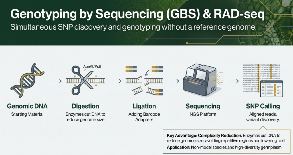
• Genotyping-by-Sequencing (GBS): A highly scalable and cost-effective method that uses restriction enzymes to reduce genome complexity. It is a “roadmap” for studying non-model species.

• Restriction-site Associated DNA Sequencing (RAD-Seq): Identifies thousands of SNPs randomly distributed across the genome by sequencing DNA fragments adjacent to restriction sites. Variants like 2b-RAD utilize type IIB endonucleases for fine-scale population studies.

• Single Locus Amplified Fragment Sequencing (SLAF-seq): An accurate and highly efficient method for large-scale SNP marker identification and genotyping.

• Targeted GBS and GT-seq: Technologies like GT-seq (Genotyping-in-Thousands by sequencing) use custom amplicon sequencing to provide highly accurate and multiplexed genotyping.

Array and Chip-Based Platforms

Arrays are preferred for projects requiring a fixed set of markers across large populations.

• Illumina BeadArray: Includes the GoldenGate and Infinium assays. These can genotype from 1,500 to over 1.1 million SNPs in parallel.

• Affymetrix Axiom: High-density arrays often used for genome-wide association studies (GWAS) and genomic selection, with capacities exceeding one million SNPs.

• DNA Chips/Microarrays: Use tiled array schemes and photolithography to achieve extremely high probe densities for reliable genotyping.

PCR-Based High-Throughput Assays

These methods are ideal for targeted genotyping of fewer SNPs across many samples.

• KASP (Kompetitive Allele-Specific PCR): A robust, single-plex method based on competitive binding of two allele-specific forward primers. It is widely used in crop breeding for its adaptability and cost-effectiveness.

• TaqMan and OpenArray: Uses 5′ exonuclease activity to degrade fluorescent probes for allele-specific discrimination. The OpenArray platform utilizes miniaturized plates to process up to 3,072 assays per plate.

• High-Resolution Melting (HRM): A post-PCR technique that identifies single-nucleotide differences by analyzing unique DNA melting curve profiles.

Mass Spectrometry and Other Analytical Methods

• MassARRAY System (iPLEX): A medium-to-high-throughput system that uses MALDI-TOF mass spectrometry to discriminate PCR extension products based on their mass.

• MALDI-TOF Mass Spectrometry: Provides high levels of automation and accuracy by determining the precise mass of DNA fragments after single-base extension.

• Pyrosequencing: A rapid re-sequencing technology that monitors nucleotide incorporation through the release of pyrophosphate, allowing for accurate scoring of SNPs.

3. Explain how SNP markers accelerate crop and animal improvement.

SNP markers accelerate crop and animal improvement by providing a high-throughput, cost-effective, and precise way to link genetic variation directly to desirable traits. As the most abundant form of DNA variation in genomes, SNPs allow researchers to identify genomic regions regulating important traits much faster and more accurately than traditional breeding methods.

High-Throughput Automation and Cost-Efficiency

The primary way SNP markers accelerate improvement is through their suitability for high-throughput and ultra-high-throughput automation.

• Massive Parallelism: Technologies like next-generation sequencing (NGS) and DNA microarrays allow thousands or millions of SNPs to be analyzed simultaneously in a single reaction.

• Reduced Costs: Modern techniques such as genotyping-by-sequencing (GBS) have significantly lowered the cost per data point, enabling the screening of large populations that would be prohibitively expensive with older markers like microsatellites or RFLPs.

• Standardized Pipelines: Advanced bioinformatics tools have simplified SNP discovery and analysis, even for “non-model” species that lack a full reference genome.

High-Resolution Mapping and Gene Discovery

Because SNPs are ubiquitous and occur at high frequencies (e.g., every 248 bp in certain rice genes), they enable the construction of saturated genetic maps with the highest possible resolution.

• Pinpointing Traits: This density allows breeders to narrow down quantitative trait loci (QTLs) to very small genomic intervals, facilitating the identification of “perfect” markers—the actual causative mutations responsible for a trait.

• Functional Understanding: SNPs located in coding or regulatory regions (cSNPs and rSNPs) help researchers understand how specific genetic changes affect protein function, gene expression, and overall phenotype.

Precision Breeding Strategies

SNPs underpin modern molecular breeding techniques that drastically reduce the time needed to develop new varieties:

• Marker-Assisted Selection (MAS): Breeders can screen plants at the seedling stage for desired alleles (such as disease resistance or high yield), saving the years of labor and field space required to wait for mature phenotypic expressions. This can reduce a 25-year conventional breeding cycle to as little as 7 to 8 years.

• Genomic Selection (GS): High-density SNP coverage allows the calculation of Genomic Estimated Breeding Values (GEBV) for all individuals in a population. This enables the selection of superior lines without needing to perform phenotypic trials in every breeding cycle.

• Gene Pyramiding: SNPs facilitate the simultaneous selection of multiple beneficial genes (e.g., resistance to several different pathogens) in a single lineage.

Applications in Crop and Animal Improvement

The sources highlight several specific areas where SNPs have made a major impact:

• Abiotic and Biotic Stress: SNPs have been used to identify resistance genes for viral, bacterial, and fungal diseases (e.g., late blight in potato, rust in wheat) and tolerance to environmental stresses like drought, salt, and heat.

• Quality and Yield: In crops like rice, maize, and soybean, SNPs have been linked to grain weight, oil content, micronutrient concentration, and flowering time.

• Animal Traceability and Management: In animal genetics, SNPs provide digital DNA signatures for individual traceability and tagging. They also improve the accuracy of paternity testing and pedigree reconstruction, which is essential for managing effective population sizes and avoiding inbreeding in breeding programs.

• Germplasm Characterization: SNPs allow breeders to mine wild relatives and ancient landraces for novel, beneficial alleles that can be introgressed into elite breeding lines.

4. What are the primary differences between SNP and SSR markers?

The primary differences between Single Nucleotide Polymorphism (SNP) and Simple Sequence Repeat (SSR or microsatellite) markers stem from their physical structure, frequency in the genome, mutation rates, and technical suitability for automation.

The following table and detailed sections summarize these differences based on the provided sources:

Summary Comparison Table

Feature	SSR Markers (Microsatellites)	SNP Markers
Structure	Tandem repeats of 1–6 base pairs	Single base pair changes (A, T, C, or G)
Allelism	Multi-allelic (highly informative per locus)	Typically bi-allelic (only two versions)
Abundance	Relatively low frequency in the genome	Most abundant and ubiquitous variation
Mutation Rate	High (10 to 100 thousand times higher than SNPs)	Low and extremely stable
Throughput	Medium (sizing alleles is laborious)	Ultra-high (fully automated genotyping)
DNA Quality	Requires larger intact DNA fragments	Suitable for degraded/historical DNA
Adaptive Signal	Primarily neutral (non-expressed regions)	Can detect both neutral and adaptive variation

1. Allelism and Information Content

• SSRs: These are multi-allelic co-dominant markers. Because a single SSR locus can have many different alleles based on the number of repeats, they provide high levels of information and heterozygosity per locus.

• SNPs: These are usually bi-allelic co-dominant markers. Because they typically represent only two possible nucleotides at a site, a much larger number of SNPs is required to reach the same statistical power as a small set of SSRs.

2. Genomic Abundance and Distribution

• SNPs: They are the most frequent form of variation in genomic DNA. They occur roughly every 100–540 base pairs in complex plant genomes like wheat and oil palm.

• SSRs: These are less frequent, occurring approximately every 10,000 base pairs in the wheat genome. While they are distributed across the whole genome, they are predominantly found in non-repetitive DNA in plants.

3. Mutation Rates and Evolutionary Resolution

• SSRs: They evolve rapidly due to replication slippage, with mutation rates estimated between 10−2 and 10−4 per generation. This makes them ideal for detecting recent demographic events, fine-scale population structure, and migration patterns occurring over short timeframes (e.g., 50–150 years).

• SNPs: They have much lower mutation rates (roughly 1×10−9), making them very stable across generations. Consequently, SNPs are better suited for studying ancient divergence and long-term evolutionary history.

4. Technical Efficiency and Automation

• SNPs: Their biggest advantage is suitability for ultra-high-throughput automation. Scoring is a simple YES/NO problem (allele presence or absence), which eliminates human error in data reading.

• SSRs: Genotyping is more laborious, requiring PCR followed by gel or capillary electrophoresis for allele size determination. This process is prone to inconsistencies between laboratories due to sizing errors and different software calling systems.

5. Selection and Functional Utility

• SNPs: Abundant in both coding and non-coding regions, they are powerful tools for identifying adaptive genetic diversity and “perfect” markers causally linked to agronomic traits.

• SSRs: generally occur in non-expressed regions and are typically considered selectively neutral. While functionally relevant SSRs in coding regions have been reported, they are less common than SNPs for gene discovery.

5. Explain how high-throughput genotyping platforms speed up genetic research.

High-throughput (HTP) genotyping platforms speed up genetic research by enabling the simultaneous analysis of massive amounts of genetic variation across large populations at a fraction of the time and cost required by traditional methods. These technologies have transformed genetic analysis into a rapid, automated, and highly scalable process.

The following sections detail how these platforms accelerate research:

1. Massive Parallelism and Throughput

Modern HTP platforms, particularly Next-Generation Sequencing (NGS) and microarrays, allow researchers to read thousands to millions of genetic markers simultaneously.

• Parallel Analysis: Array-based platforms like Illumina’s BeadArray can genotype from 1,500 to over 1.1 million SNPs in parallel.

• Concurrent Discovery and Genotyping: Methods such as Genotyping-by-Sequencing (GBS) and RAD-Seq allow for the simultaneous discovery and analysis of millions of SNPs, eliminating the need for prior genomic knowledge in non-model species.

• Rapid Acquisition: Certain technologies, such as MALDI-TOF mass spectrometry, can acquire genotypes in just a few seconds per data point.

2. Automation and Standardized Pipelines

The shift toward HTP platforms has moved genetic research away from laborious, manual processes toward fully automated laboratory and bioinformatics workflows.

• Reduced Labor: Automation minimizes human manipulation errors and dramatically increases the speed of data generation.

• Bioinformatics Efficiency: Standardized computational pipelines can process raw sequencing data into usable genetic information in a few hours, even when analyzing numerous species at once.

• Simplified Allele Scoring: Unlike older markers like microsatellites that require complex “allele sizing,” SNPs are scored as a simple YES/NO (bi-allelic) problem, which is far easier for software to analyze automatically.

3. Accelerated Gene/QTL Discovery

The high density of markers provided by HTP platforms allows researchers to identify Quantitative Trait Loci (QTLs) and causative genes with unprecedented speed and precision.

• Fine-Scale Mapping: High-density SNP maps can narrow down a trait’s location from a massive multi-megabase region to a very small interval (e.g., 123 kb) in a single study.

• Marker-Assisted Selection (MAS): HTP platforms enable breeders to screen for desirable traits at the seedling stage rather than waiting for maturity. This can reduce a 25-year conventional breeding cycle to as little as 7 to 8 years.

4. Cost Efficiency and Scalability

By significantly lowering the cost per data point, HTP platforms allow for research projects of a scale that was previously impossible.

• Larger Populations: Lower costs enable the analysis of much larger population samples, which increases the statistical power to detect rare or complex genetic variants.

• Resource Allocation: Technologies like TaqMan OpenArray can process over 3,000 individual assays on a single miniaturized plate, maximizing data output while minimizing reagent use.

5. Rapid Research in “Non-Model” Species

HTP platforms have removed the “bottleneck” of needing a pre-existing reference genome for every species under study.

• Reference-Free Discovery: New reference-free approaches can detect SNPs directly from raw sequencing reads, allowing for immediate research into the population structure or history of orphan or wild species.

• Genome Complexity Reduction: Techniques like SLAF-seq or CRoPS filter out repetitive DNA to focus only on informative genetic regions, speeding up the identification of markers in complex, high-repeat genomes

6. How are SNP markers used to characterize ancient crop landraces?

SNP markers are instrumental in characterizing ancient crop landraces by providing high-resolution genomic data that reveals their unique genetic structure, evolutionary history, and reservoirs of beneficial traits. Because landraces are often genetically unique, diverse, and adapted to specific regional ecotypes, they serve as critical resources for modern breeding.

The following sections detail how SNP markers are used for these characterizations:

1. Assessing Genetic Diversity and Relationships

SNP markers are used to quantify the “hyper-variable” nature of ancient landraces compared to modern elite cultivars.

• Unique Genetic Signatures: Landraces often possess high levels of genetic variation due to centuries of natural and human selection in diverse agro-ecologies. For instance, SNP analysis of Ethiopian barley landraces revealed substantial genetic variation, which is critical for identifying unique ancestry and managing crop genetic resources.

• Population Structure: By analyzing thousands of SNPs simultaneously, researchers can identify distinct clusters or subpopulations within a collection of landraces. This helps in assigning individuals into heterotic groups or identifying specific inbred lines.

2. Tracing Domestication and Evolutionary History

Comparing the genotypes of ancient landraces with those of wild relatives and modern cultivars allows researchers to “unravel the molecular mechanism of evolution”.

• Domestication Footprints: SNPs can pinpoint specific mutations that were intentionally selected during a crop’s transition from wild to domesticated forms. A prominent example is the identification of a single SNP in the regulatory region of the qSH1 gene in rice, which was found to be responsible for the loss of seed shattering—a key domestication trait.

• Ancestry Analysis: SNP data can reveal the breeding history and relationships among landraces, identifying how they have diverged over time due to geographical isolation and varying environmental factors.

3. Mining Beneficial and Adaptive Alleles

Ancient landraces are frequently characterized as “significant sources of disease-resistant genes” and other adaptive traits that may have been lost in modern high-yielding varieties.

• Functional Polymorphisms: Researchers use SNP markers to identify “outlier” loci—genomic regions under strong natural selection. These often represent local adaptations to climate, pests, or specific pathogens.

• Introgression: Once beneficial SNPs (such as those for drought tolerance or disease resistance) are identified in landraces, they can be precisely tracked as they are “introgressed” into elite breeding lines through Marker-Assisted Selection (MAS).

4. Conservation and Germplasm Management

Characterizing landraces with SNPs is essential for effective germplasm conservation.

• Identifying Redundancy: Genomic data helps curators eliminate duplicates in gene banks, ensuring that unique genetic diversity is preserved efficiently.

• Prioritizing Targets: By mapping the genetic distance and identity between various landraces, conservationists can prioritize ancient varieties that harbor the most unique genetic components for long-term storage and protection.

7. How do KASP and TaqMan assays handle specific traits?

KASP (Kompetitive Allele-Specific PCR) and TaqMan assays handle specific traits by targeting and discriminating between individual single nucleotide polymorphisms (SNPs) that are causally linked or tightly associated with those traits. These assays function as high-throughput, single-plex genotyping tools, meaning they are designed to analyze a few specific markers across many different samples.

Technical Handling of Trait Discrimination

Both assays rely on fluorescent signaling to identify the presence of specific alleles associated with a trait:

• TaqMan Assays: These use a 5′ exonuclease activity to degrade an internal fluorescent probe that contains a reporter and a quencher. Allele-specific discrimination is achieved by using two different internal probes, each labeled with a different color (e.g., VIC and FAM), which bind only when there is a perfect match to the target trait sequence.

• KASP Assays: These utilize competitive binding of two allele-specific forward primers. Like TaqMan, they use fluorescent resonant energy transfer (FRET) for detection, where a signal is emitted only when a specific primer successfully binds to and amplifies the DNA sequence containing the trait-linked allele.

Specific Traits Handled by These Assays

According to the sources, these technologies are used to track a wide range of critical agronomic and health-related traits:

• Disease and Pathogen Resistance:

    ◦ In tomato, they are used to identify resistance-breaking isolates of Tomato Spotted Wilt Virus (TSWV) and to differentiate between resistant and susceptible alleles for Tomato Mosaic Virus (ToMV) at the Tm-2 and Tm-22 loci.

    ◦ In wheat, these assays target the Fhb1 gene for Fusarium head blight resistance and the Lr34/Yr18/Pm38 locus for resistance to leaf rust, stripe rust, and powdery mildew.

    ◦ In soybean, they identify markers linked to root-knot nematode resistance and aphid resistance genes (Rag1 and Rag2).

• Abiotic Stress Tolerance:

    ◦ KASP has been specifically used to validate SNPs linked to heat stress tolerance in maize and salt tolerance in barley and soybean.

    ◦ Assays also target genes like IbOr in sweet potato, where a unique SNP is associated with both carotenoid accumulation and enhanced heat stress tolerance.

• Quality and Composition Traits:

    ◦ In cassava, KASP markers are used to select for high provitamin A carotenoid content by targeting the phytoene synthase 2 gene.

    ◦ In canola, these assays discriminate between alleles of the fad2 and fad3 genes to control oleic and linolenic acid content.

    ◦ In sorghum, they are used to identify the brown midrib (bmr) trait at the seedling stage, which affects the plant’s nutritional quality.

• Morphological Traits:

    ◦ Assays track the TAC1 gene in rice, which controls the tiller angle crucial for achieving high yields.

    ◦ They are also used in upland cotton to genotype the GhOKRA gene, which regulates leaf morphology.

Advantages for Applied Breeding

By using these assays to handle specific traits, breeders can implement Marker-Assisted Selection (MAS) at the seedling stage. This eliminates the need to wait for a plant to reach maturity to observe its physical characteristics, drastically reducing breeding cycle times. Because these assays provide a simple YES/NO result regarding the presence of a target allele, they minimize human error and allow for high levels of automation.

8. What challenges do polyploid genomes present for SNP discovery?

Polyploid genomes—those containing more than two sets of chromosomes—present significant hurdles for SNP discovery primarily because of their high level of sequence duplication and the presence of multiple subgenomes.

The primary challenges identified in the sources include:

1. Distinguishing True SNPs from Subgenome Variants

The most fundamental challenge is differentiating “true” SNPs (variations between individuals at the same locus) from homoeologous sequence variants (HSVs) or paralogous variations.

• False Positives: In polyploids like wheat or cotton, loci may appear polymorphic within a single genotype simply because the assay is detecting differences between subgenomes (e.g., A subgenome vs. D subgenome) rather than differences between individuals.

• Low “True” SNP Rate: In some species like the cultivated peanut, the ancestral subgenomes diverged millions of years ago, while the cultivated varieties diverged only thousands of years ago. This means “false” A-vs-B genome variations can be 1,000 times more frequent than the true SNPs breeders need to track.

2. Genotyping Signal Interference

Standard genotyping assays designed for diploids often struggle with the “interfering signal” generated by DNA bases from other subgenomes.

• Distorted Plots: Assays that normally distinguish two versions of a base (e.g., G and T) may detect four or more bases in a polyploid, leading to distorted signal intensity plots that standard software cannot automatically score.

• Complex Allelic States: In autopolyploids like potato, five different genotypic states are possible at a single locus (ranging from zero to four copies of an allele), which is far more complex than the three states found in diploids.

3. Complexity and Repetitiveness

Many polyploid species, particularly conifers and certain crops like wheat, possess humongous and highly repetitive genomes.

• Assembly Difficulties: High repeat content makes it difficult to achieve accurate de novo assembly or to align short reads correctly. Reads from similar but non-identical genomic regions may map “on top of each other,” leading to false variant calls.

• Incomplete References: Because of their massive size (often ≥ 18–20 Gb), most polyploid reference genomes are incomplete, which complicates the mapping process necessary for SNP discovery.

4. Specialized Bioinformatic and Experimental Needs

Standard filters used for diploids, such as minor allele frequency (MAF), are often insufficient for polyploids.

• Haplotype Requirement: Distinguishing homologous SNPs from homoeologous ones often requires using haplotype information rather than just allele frequency.

• Specific Primer Design: To isolate true SNPs in species like hexaploid wheat, researchers must often design primers where the 3′-end matches a known subgenome-specific variant (HSV) to ensure they are amplifying only one of the three subgenomes.

9. How does GBS reduce genome complexity for faster genotyping?

Genotyping-by-Sequencing (GBS) reduces genome complexity primarily by employing a reduced-representation genome sequencing approach, which allows researchers to focus on a manageable subset of the total DNA rather than sequencing every base pair.

The following sections detail how this complexity reduction facilitates faster and more efficient genotyping:

1. Targeted Digestion with Restriction Enzymes

The core mechanism of GBS is the use of restriction enzymes (such as ApeKI, PstI, or HpaII) to digest genomic DNA at specific, predictable recognition sites. This process targets specific intervals of the genome, effectively filtering out a large portion of highly repetitive sequences that often confound genetic analysis in complex genomes. By creating these “reduced representation libraries,” sequencing efforts are concentrated on a fraction of the total genome.

2. Massively Parallel Sequencing

Because the amount of DNA to be read is significantly reduced, GBS allows for massive parallelism and high throughput. Thousands of SNP markers can be identified and scored simultaneously across hundreds of individuals in a single sequencing run. This process is much faster than older methods that require laborious PCR and electrophoresis for individual loci.

3. Technical and Economic Efficiency

GBS speeds up research by providing a “roadmap” for non-model species that lack a full reference genome. The technology offers:

• Rapid Data Acquisition: Genotyping that once took years through conventional breeding cycles can be completed in just a few days.

• Lower Costs: The simple methodology and reduced data requirements significantly lower the cost per data point, making large-scale population studies financially viable.

• Multiplexing Capabilities: Modern GBS protocols can multiplex up to 384 samples in a single run, maximizing data output.

4. Streamlined Bioinformatics Analysis

The reduction in genome complexity also simplifies the computational task of variant calling. Because the sequenced fragments are tied to specific restriction sites, bioinformatic pipelines can more easily align reads and identify single-base variations. In some designs, once the raw data is treated, the automatic pipeline implementation can be performed in just a few hours on standard cluster nodes.

10. Which SNP genotyping platforms are best for small-scale research projects?

For small-scale research projects, the best SNP genotyping platforms are those that offer cost-effectiveness, flexibility in marker/sample numbers, and minimal requirements for specialized bioinformatics infrastructure. Based on the sources, the following platforms are most suitable:

1. KASP (Kompetitive Allele-Specific PCR)

KASP is frequently highlighted as a robust, easy-to-use, and highly adaptable method for small-scale projects.

• Cost-Effectiveness: It is widely applied because of its reduced cost, particularly when genotyping a small number of SNPs across a population.

• Accessibility: It is compatible with standard laboratory equipment and does not require complex probe synthesis, making it more accessible for academic labs.

2. MassARRAY (iPLEX) System

For projects involving a limited number of samples (e.g., hundreds rather than thousands), the MassARRAY system is often more affordable than targeted sequencing technologies like GT-seq or Tru-Seq.

• Tractability: The data outputs are easily managed using classical spreadsheet formats, eliminating the need for high-level bioinformatics skills or calculation clusters required by GBS.

• Throughput: It is efficient for analyzing between 100 and 500 SNPs per species at a cost of approximately $30 per sample.

3. TaqMan and OpenArray

TaqMan assays are ideal for targeted applications where researchers need to track a specific set of QTLs across many samples.

• Synthesis Speed: TaqMan assays can be synthesized much faster (c. 2 weeks) than larger array platforms like GoldenGate (6 weeks) or Infinium (9 weeks).

• Flexibility: While high-density arrays are better for genome-wide studies, the OpenArray platform is more suitable for scenarios involving fewer SNPs and larger sample populations.

4. Tetra ARMS (Amplification Refractory Mutation System) PCR

This is the most economical and baseline tool for very small-scale or low-to-moderate throughput situations.

• Minimal Equipment: It requires only a single PCR step followed by gel electrophoresis, making it possible to conduct research without expensive specialized scanners or mass spectrometers.

Platforms to Exercise Caution With

While powerful, high-density arrays (like Illumina’s GoldenGate or Infinium) may be unsuitable for small-scale research because they often have minimum sample requirements (e.g., 480 to 1,152 samples) to be cost-effective. Similarly, while GBS (Genotyping-by-Sequencing) is low-cost per data point, it requires access to bioinformatics expertise and computing clusters, which may exceed the resources of a small research project.

11. How are machine learning models used to select true SNPs?

Machine learning models are increasingly being used to select true SNPs by providing intelligent decision-making on the accuracy of detected polymorphisms, specifically to address the high rate of false-positive SNPs generated by some next-generation sequencing (NGS) analysis tools.

According to the sources, these models offer the following functionalities:

• Direct Selection from Sequence Data: Machine learning represents a groundbreaking approach to selecting true SNPs directly from raw sequence data rather than relying solely on traditional binary compositions of nucleotides.

• Addressing Bulk Data Challenges: There is a growing need for tools that can extract vast amounts of data and support complex analyses; machine learning helps fulfill this by automating the identification of high-quality variants in large-scale datasets.

• Integrated Mining Pipelines: One of the first significant trials in this area is the Integrated SNP Mining and Utilization (ISMU) Pipeline, which was developed as a machine learning approach to SNP discovery to improve reliability and reduce the error-prone nature of standard NGS pipelines.

• Specialized Screening Applications: Machine learning has been applied to specific research goals, such as the screening of aquaculture-associated introgression into at-risk wild Atlantic salmon populations in North America.

By integrating these models with recent innovations in sequencing technology, researchers can gain deeper insights into evolutionary and genetic relationships while minimizing the technical artifacts that often plague high-throughput genomic studies.

12. What causes the higher frequency of transition vs transversion mutations?

The higher frequency of transition mutations compared to transversions—often occurring at a ratio of 1.5:1 to 4:1 depending on the species—is primarily caused by specific biochemical mechanisms and evolutionary selection pressures.

According to the sources, the following factors contribute to this bias:

1. Spontaneous Chemical Deamination

The most significant biochemical cause for the prevalence of transitions is the high spontaneous rate of deamination of 5-methylcytosine (5mC) to thymidine within CpG dinucleotides.

• This specific chemical reaction leads to a high frequency of C ⇔ T transitions (which appear as G ⇔ A transitions on the reverse DNA strand).

• Because this deamination occurs frequently and spontaneously, it generates transitions at a much higher rate than the random mutations that cause transversions.

2. Structural Stability and Ease of Substitution

From a molecular perspective, transitions are simply “easier” and more stable to produce than transversions.

• Transitions involve substituting a base with another of the same chemical structure (a purine for a purine, like A ⇔ G, or a pyrimidine for a pyrimidine, like C ⇔ T).

• Transversions require swapping a purine for a pyrimidine (or vice versa), which is a more complex structural change that is less chemically stable and less likely to occur.

3. Evolutionary Conservation of Proteins

Transitions are more common in surviving lineages because they tend to be more conservative in their effects on proteins.

• Because transition mutations are less likely than transversions to result in a radical change to the encoded amino acid, they are less likely to be harmful to the organism.

• As a result, transitions are more frequently tolerated by natural selection and accumulate in the genome over time.

Summary of Differences

While there are twice as many possible transversion paths as there are transition paths (8 possible transversions vs. 4 possible transitions), the actual observed data consistently shows a bias toward transitions due to these chemical and biological advantages. If mutations were truly random, researchers would expect a transition-to-transversion ratio of 1:2, but the biological reality is closer to 2:1 for vertebrates.

13. How do CpG dinucleotides influence the transition-to-transversion bias?

CpG dinucleotides significantly influence the transition-to-transversion bias through a specific biochemical mechanism involving spontaneous chemical deamination.

The primary ways this influence occurs include:

• Deamination of 5-methylcytosine: The most probable explanation for the bias toward transitions is the high spontaneous rate of deamination of 5-methylcytosine (5mC) to thymidine within CpG dinucleotides.

• Generation of Specific Transitions: This chemical reaction directly generates C ⇔ T transitions. Because DNA is double-stranded, these mutations are observed as G ⇔ A transitions on the reverse strand.

• Skewing the Ratio: While there are twice as many possible transversion paths (eight) as there are transition paths (four), this frequent deamination at CpG sites ensures that transitions occur much more often in practice. If mutations were purely random, the ratio would be 0.5, but due to this effect, observed ratios are typically much higher, such as 1.5:1 to 2.5:1 in many organisms and up to 4:1 in some species like chickens.

Beyond the chemical deamination at CpG sites, this bias is further reinforced by natural selection, as transition mutations tend to be more conservative in their effects on protein sequences, making them less likely to be harmful and more likely to be preserved in the genome.

14. Are transitions less harmful to protein function than transversions?

Yes, transitions are generally less harmful to protein function than transversions because they tend to be more conservative in their effects on the encoded amino acids.

The following factors explain why transitions are less deleterious:

• Conservative Amino Acid Changes: Transition mutations are less likely than transversions to result in a radical change to the chemical properties of an amino acid. Because they often result in no change (synonymous mutation) or a change to a chemically similar amino acid, they are less likely to disrupt the overall structure or function of a protein.

• Tolerance by Natural Selection: Due to their relatively mild impact on protein function, transitions are more frequently tolerated by natural selection. This allows them to accumulate in surviving lineages and contribute to the observed bias where transitions occur at a much higher frequency than transversions.

• Structural Stability: From a molecular standpoint, a transition—which involves replacing a base with another of the same structural class (a purine for a purine or a pyrimidine for a pyrimidine)—is a more stable and “easier” substitution than a transversion, which requires swapping between classes.

In contrast, transversions involve a more complex structural change (purine-to-pyrimidine or vice-versa) that is more likely to cause a significant amino acid substitution. Although there are twice as many possible transversion paths (8) as transition paths (4), the biological and chemical advantages of transitions lead to a consistent bias in nature, often observed at a ratio of 2:1 in vertebrates.

15. How do SNPs help mine rare alleles from wild germplasm?

SNPs help mine rare alleles from wild germplasm by providing the high density and genomic resolution necessary to pinpoint specific, often unique, genetic variations that have been lost in modern cultivars during domestication. Because wild relatives and ancient landraces serve as significant reservoirs for disease resistance and environmental adaptation genes, SNPs act as precise tools to identify and extract these beneficial traits.

The process through which SNPs facilitate this mining includes:

1. High-Resolution Mapping of Desirable Traits

Because SNPs are the most abundant form of DNA variation, they allow researchers to construct saturated genetic maps that can narrow down a trait’s location to extremely small genomic intervals.

• Pinpointing Causative Mutations: This precision enables the identification of “perfect” markers—the actual functional polymorphisms responsible for a trait, such as the single SNP found to control seed shattering in rice domestication.

• Narrowing QTL Intervals: In soybean, SNPs were used to narrow the mapping interval for aphid resistance genes from large 10 cM regions down to precise 54 kb and 115 kb intervals.

2. Efficient Screening of Large Germplasm Collections

Wild germplasm collections can be massive, but modern high-throughput technologies make scanning them for rare alleles economically viable.

• Genotyping-by-Sequencing (GBS): Technologies like GBS allow for the rapid discovery of millions of SNPs across thousands of wild accessions without needing a prior reference genome, making it easier to capture the genetic variability of a species.

• Mining “Outlier” Loci: By analyzing thousands of markers simultaneously, researchers can identify “outlier” SNPs that show signatures of natural selection, which often correspond to local adaptations for heat, salt, or drought tolerance in wild populations.

3. Precise Tracking during Introgression

Once beneficial rare alleles are identified in wild germplasm, SNPs are used to monitor their transfer into elite breeding lines through Marker-Assisted Selection (MAS).

• Early-Stage Selection: Breeders can screen seedlings for the presence of the specific wild allele, saving years of labor by avoiding the need to wait for the plant to reach phenotypic maturity.

• Gene Pyramiding: SNPs facilitate the simultaneous selection of multiple rare alleles (e.g., resistance to several different pathogens) from different wild sources into a single variety.

4. Characterizing Genetic Structure and Relationships

SNPs help quantify the high levels of variation in wild germplasm, which is essential for strategic parental selection and managing genetic resources.

• Identifying Unique Ancestry: For example, SNP analysis of Ethiopian barley genotypes confirmed substantial genetic variation that can be valorized to develop new varieties with high yield and stress tolerance.

• Conservation Management: Genomic data helps curators eliminate redundancy in gene banks and prioritize wild varieties that harbor the most unique genetic components for long-term storage.

16. How can homoeologous sequence variants be distinguished from true SNPs?

Distinguishing homoeologous sequence variants (HSVs)—which are variations between subgenomes within a single individual—from true SNPs—which are variations between different individuals at the same locus—is a critical challenge in polyploid genetics. In hexaploid wheat, for instance, HSVs occur at a much higher frequency (1 per 24 bp) than true SNPs (1 per 540 bp), making differentiation essential for reliable genotyping.

The following strategies are used to distinguish these variants based on the sources:

1. Specific Primer Design

A primary experimental method involves designing locus-specific primers that target both a true SNP and a known HSV.

• 3′-End Matching: Researchers design a pair of primers where the 3′-end nucleotide of one primer matches the true SNP, and the 3′-end of the other primer matches the nearest known HSV.

• Subgenome Isolation: By matching the 3′-end to a subgenome-specific variant (HSV), the PCR reaction is forced to amplify only one of the subgenomes, ensuring that any subsequent polymorphism detected is a true SNP.

2. Bioinformatic and Statistical Approaches

Several “in silico” methods allow for the separation of these variants without the need for initial laboratory amplification:

• Haplotype Analysis: Using bioinformatic programs like HaploSNPer allows researchers to use haplotype information rather than just allele frequency to identify homologous SNPs.

• Software Pipelines: Programs like PHRAP can perform statistical analysis on overlapping EST sequences to distinguish between wheat SNPs and HSVs.

• Reference-Free Mapping: Tools such as ebwt2InDel can detect variants directly from raw reads by using positional clustering to locate genome positions where reads from different genotypes differ, which helps filter out subgenome-specific noise in the absence of a reference genome.

3. Signal Analysis in Genotyping Assays

In high-throughput platforms like Illumina’s GoldenGate, the presence of subgenomes creates an “interfering signal” that can be identified and corrected:

• Distorted Intensity Plots: Because assays often detect four DNA bases in a tetraploid instead of two, the resulting signal intensity plots are “distorted” compared to diploid patterns.

• Manual Cluster Correction: Software like GenomeStudio allows experts to identify these distorted clusters. For example, if a base is monomorphic in the B genome but polymorphic in the A genome (e.g., GG:GG vs TG:GG), the excess of the monomorphic base shifts the genotype clusters at a specific angle, which can then be manually corrected to call the true A-genome SNP.

4. Use of Diploid Progenitors

Comparing polyploid sequences against their closely related diploid ancestors provides a clear baseline for what constitutes a subgenome difference.

• Subgenome Mapping: By genotyping both the polyploid and its diploid ancestors (e.g., A and D subgenome progenitors for cotton), researchers can identify “Homoeo-SNPs” that are monomorphic between tetraploid varieties but differ between the original subgenomes.

• Hemi-SNP Detection: This identifies variants that appear homozygous in one sample and heterozygous in another, signaling a variation in one subgenome while the other remains stable.

5. Transition-to-Transversion (Ts/Tv) Ratio

Monitoring the Ts/Tv ratio acts as a quality control measure. A significant amount of false-positive variants (which often includes incorrectly identified HSVs) would lead to random permutations between all four nucleotides, causing the ratio to fall toward 1:2. A ratio closer to 2:1 in vertebrates or 1.5:1 in invertebrates indicates a higher proportion of true biological transitions, suggesting the identified markers are likely true SNPs rather than sequencing artifacts or misaligned homoeologs.

References

Anokye, B., Amoah, P., Potter Jr, B. W., & Olasanmi, B. (2025). The Role of Single Nucleotide Polymorphisms (SNPs) in Modern Plant Breeding: From Discovery to Application. https://doi.org/10.20944/preprints202504.1646.v1
Bertioli, D. J., Ozias-Akins, P., Chu, Y., Dantas, K. M., Santos, S. P., Gouvea, E., Guimarães, P. M., Leal-Bertioli, S. C. M., Knapp, S. J., & Moretzsohn, M. C. (2014). The use of SNP markers for linkage mapping in diploid and tetraploid peanuts. G3: Genes, Genomes, Genetics, 4(1), 89–96. https://doi.org/10.1534/g3.113.007617
Das, D., & Mishra, R. (2022). SNP Markers and its Impact on Crop Improvement. Asian Journal of Biological and Life Sciences, 539–548. https://doi.org/10.5530/ajbls.2021.10.72
Delord, C., Lassalle, G., Oger, A., Barloy, D., Coutellec, M. A., Delcamp, A., Evanno, G., Genthon, C., Guichoux, E., Le Bail, P. Y., Le Quilliec, P., Longin, G., Lorvelec, O., Massot, M., Reveillac, E., Rinaldo, R., Roussel, J. M., Vigouroux, R., Launey, S., & Petit, E. J. (2018). A cost-and-time effective procedure to develop SNP markers for multiple species: A support for community genetics. Methods in Ecology and Evolution, 9(9), 1959–1974. https://doi.org/10.1111/2041-210X.13034
Dwiningsih, Y., Rahmaningsih, M., & Alkahtani, J. (2020). Development of Single Nucleotide Polymorphism (SNP) Markersin Tropical Crops. Advance Sustainable Science, Engineering and Technology, 2(2). https://doi.org/10.26877/asset.v2i2.6279
Hakim, I. R., Kammoun, N. G., Makhloufi, E., & Rebaï, A. (2010). Discovery and potential of SNP markers in characterization of Tunisian olive germplasm. Diversity, 2(1), 17–27. https://doi.org/10.3390/d2010017
I. Udoh, L., Peggy Obaseojei, W., & Uzoebo, C. (2021). Single Nucleotide Polymorphisms: A Modern Tool to Screen Plants for Desirable Traits. In Plant Breeding – Current and Future Views. IntechOpen. https://doi.org/10.5772/intechopen.94935
Khlestkina, E. K., & Salina, E. A. (2006). SNP markers: Methods of analysis, ways of development, and comparison on an example of common wheat. In Russian Journal of Genetics (Vol. 42, Number 6, pp. 585–594). https://doi.org/10.1134/S1022795406060019
Kim, J. E., Lee, Y. M., Lee, J.-H., Noh, J. K., Kim, H. C., Park, C.-J., Park, J.-W., & Kim, K.-K. (2014). Development and Validation of Single Nucleotide Polymorphism (SNP) Markers from an Expressed Sequence Tag (EST) Database in Olive Flounder (Paralichthys olivaceus). Development & Reproduciton, 18(4), 275–286. https://doi.org/10.12717/dr.2014.18.4.275
Kundu, V. (2022). SNP Genotyping: A Revolutionary Tool for Crop Improvement. www.biospub.com
Mammadov, J., Aggarwal, R., Buyyarapu, R., & Kumpatla, S. (2012). SNP markers and their impact on plant breeding. In International Journal of Plant Genomics (Vol. 2012). https://doi.org/10.1155/2012/728398
Mishra, A., Singh, P. K., Bhandawat, A., Sharma, Vinay, Sharma, Vikas, Singh, P., Roy, J., & Sharma, H. (2021). Analysis of SSR and SNP markers. In Bioinformatics: Methods and Applications (pp. 131–144). Elsevier. https://doi.org/10.1016/B978-0-323-89775-4.00017-1
Morgil, H., Can Gercek, Y., & Tulum, I. (2020). Single Nucleotide Polymorphisms (SNPs) in Plant Genetics and Breeding. In The Recent Topics in Genetic Polymorphisms. IntechOpen. https://doi.org/10.5772/intechopen.91886
Ousmael, K., Whetten, R. W., Xu, J., Nielsen, U. B., Lamour, K., & Hansen, O. K. (2023). Identification and high-throughput genotyping of single nucleotide polymorphism markers in a non-model conifer (Abies nordmanniana (Steven) Spach). Scientific Reports, 13(1). https://doi.org/10.1038/s41598-023-49462-x
Tsykun, T., Rellstab, C., Dutech, C., Sipos, G., & Prospero, S. (2017). Comparative assessment of SSR and SNP markers for inferring the population genetic structure of the common fungus Armillaria cepistipes. Heredity, 119(5), 371–380. https://doi.org/10.1038/hdy.2017.48
Vignal, A., Milan, D., SanCristobal, M., & Eggen, A. (2002). A review on SNP and other types of molecular markers and their use in animal genetics. In Genetics Selection Evolution (Vol. 34, Number 3, pp. 275–305). EDP Sciences. https://doi.org/10.1051/gse:2002009
Wenne, R. (2023). Single Nucleotide Polymorphism Markers with Applications in Conservation and Exploitation of Aquatic Natural Populations. In Animals (Vol. 13, Number 6). MDPI. https://doi.org/10.3390/ani13061089
Xia, W., Luo, T., Zhang, W., Mason, A. S., Huang, D., Huang, X., Tang, W., Dou, Y., Zhang, C., & Xiao, Y. (2019). Development of high-density snp markers and their application in evaluating genetic diversity and population structure in elaeis guineensis. Frontiers in Plant Science, 10. https://doi.org/10.3389/fpls.2019.00130
Yirgu, M., Kebede, M., Feyissa, T., Lakew, B., Woldeyohannes, A. B., & Fikere, M. (2023). Single nucleotide polymorphism (SNP) markers for genetic diversity and population structure study in Ethiopian barley (Hordeum vulgare L.) germplasm. BMC Genomic Data, 24(1). https://doi.org/10.1186/s12863-023-01109-6